Page 115 - MATLAB Recipes for Earth Sciences

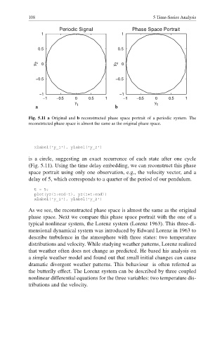
108 5 Time-Series Analysis

Periodic Signal Phase Space Portrait
1 1

0.5 0.5

y 2 0 y 2 0

−0.5 −0.5

−1 −1
−1 −0.5 0 0.5 1 −1 −0.5 0 0.5 1
y 1 y 1
a b

Fig. 5.11 a Original and b reconstructed phase space portrait of a periodic system. The
reconstructed phase space is almost the same as the original phase space.

xlabel('y_1'), ylabel('y_2')

is a circle, suggesting an exact recurrence of each state after one cycle
(Fig. 5.11). Using the time delay embedding, we can reconstruct this phase
space portrait using only one observation, e.g., the velocity vector, and a
delay of 5, which corresponds to a quarter of the period of our pendulum.
t = 5;
plot(y2(1:end-t), y2(1+t:end))
xlabel('y_1'), ylabel('y_2')
As we see, the reconstructed phase space is almost the same as the original
phase space. Next we compare this phase space portrait with the one of a
typical nonlinear system, the Lorenz system (Lorenz 1963). This three-di-
mensional dynamical system was introduced by Edward Lorenz in 1963 to
describe turbulence in the atmosphere with three states: two temperature
distributions and velocity. While studying weather patterns, Lorenz realized
that weather often does not change as predicted. He based his analysis on
a simple weather model and found out that small initial changes can cause
dramatic divergent weather patterns. This behaviour is often referred as

the butterfly effect. The Lorenz system can be described by three coupled
nonlinear differential equations for the three variables: two temperature dis-
tributions and the velocity.