Page 112 - MATLAB Recipes for Earth Sciences

5.5 Interpolating and Analyzing Unevenly-Spaced Data 105

Time Domain Cross PSD Estimate
5 700
1st data series
600
f 1 =0.01
500
y(t) 0 Power 400
300
f 2 =0.025
200
f 3 =0.05
2nd data 100
series
ï5 0
0 200 400 600 800 1000 0 0.05 0.1 0.15 0.2
t Frequency
a b
Coherence Estimate Phase spectrum
1 High coherence in 4 3 Phase angle in the 0.01
Magnitude Squared Coherence 0.6 band Phase angle ï1 2 1 0
frequency band
the 0.01 frequency
0.8

0.4

0.2
ï3
0 ï2
ï4
0 0.05 0.1 0.15 0.2 0 0.05 0.1 0.15 0.2
Frequency Frequency
c d
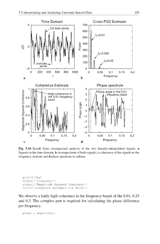
Fig. 5.10 Result from crossspectral analysis of the two linearly-interpolated signals. a
Signals in the time domain, b crossspectrum of both signals, c coherence of the signals in the
frequency domain and d phase spectrum in radians.

plot(f,Cxy)
xlabel('Frequency')
ylabel('Magnitude Squared Coherence')
title('Coherence Estimate via Welch')
We observe a fairly high coherence in the frequency bands of the 0.01, 0.25
and 0.5. The complex part is required for calculating the phase difference
per frequency.
phase = angle(Pxy);