Page 119 - MATLAB Recipes for Earth Sciences

112 5 Time-Series Analysis

Recurrence Plots

Th phase space trajectories of dynamic systems that have more than three

dimensions are difficult to visualize. Recurrence plots provide a way for
analyzing higher dimensional systems. They can be used, e.g., to detect tran-

sitions between different regimes or to find interrelations between several

systems. The method was first introduced by Eckmann and others (1987).
The recurrence plot is a tool that visualizes the recurrences of states in the
phase space by a two-dimensional plot.

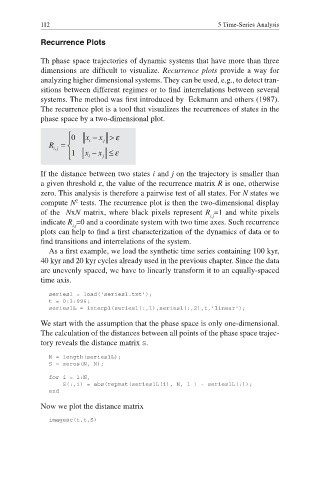
If the distance between two states i and j on the trajectory is smaller than
a given threshold ε, the value of the recurrence matrix R is one, otherwise
zero. This analysis is therefore a pairwise test of all states. For N states we
2
compute N tests. The recurrence plot is then the two-dimensional display
of the NxN matrix, where black pixels represent R =1 and white pixels
i,j
indicate R =0 and a coordinate system with two time axes. Such recurrence
i,j
plots can help to find a first characterization of the dynamics of data or to

find transitions and interrelations of the system.
As a fi rst example, we load the synthetic time series containing 100 kyr,
40 kyr and 20 kyr cycles already used in the previous chapter. Since the data
are unevenly spaced, we have to linearly transform it to an equally-spaced
time axis.
series1 = load('series1.txt');
t = 0:3:996;
series1L = interp1(series1(:,1),series1(:,2),t,'linear');

We start with the assumption that the phase space is only one-dimensional.
The calculation of the distances between all points of the phase space trajec-
tory reveals the distance matrix S.

N = length(series1L);
S = zeros(N, N);
for i = 1:N,
S(:,i) = abs(repmat(series1L(i), N, 1 ) - series1L(:));
end
Now we plot the distance matrix
imagesc(t,t,S)