Page 191 - Materials Science and Engineering An Introduction

Questions and Problems • 163

9
the diffusion flux is 7.36 10 kg/m # s. Hint: Use At what position will the carbon concentration be
2
Equation 4.9 to convert the concentrations from 0.25 wt% after a 10-h treatment? The value of D
2
weight percent to kilograms of carbon per cubic at 1325 K is 3.3 10 11 m /s.
meter of iron. 5.15 Nitrogen from a gaseous phase is to be diffused
5.11 When a-iron is subjected to an atmosphere of into pure iron at 675 C. If the surface concentra-
nitrogen gas, the concentration of nitrogen in tion is maintained at 0.2 wt% N, what will be the
(in weight percent), is a function of concentration 2 mm from the surface after 25 h?
the iron, C N
(in MPa), and absolute The diffusion coefficient for nitrogen in iron at
hydrogen pressure, p N 2
2
temperature (T) according to 675 C is 2.8 10 11 m /s.
37,600 J>mol 5.16 Consider a diffusion couple composed of two
C N = 4.90 * 10 -3 1p N 2 expa - b (5.14) semi-infinite solids of the same metal and that
RT
each side of the diffusion couple has a different
Furthermore, the values of D 0 and Q d for this diffu- concentration of the same elemental impurity; fur-
2
7
sion system are 5.0 10 m /s and 77,000 J/mol, re- thermore, assume each impurity level is constant
spectively. Consider a thin iron membrane 1.5-mm throughout its side of the diffusion couple. For this
thick at 300 C. Compute the diffusion flux through situation, the solution to Fick’s second law (assum-
this membrane if the nitrogen pressure on one side ing that the diffusion coefficient for the impurity is
of the membrane is 0.10 MPa (0.99 atm) and on the independent of concentration) is as follows:
other side is 5.0 MPa (49.3 atm).
C 1 - C 2 x
C x = C 2 + a b c 1 - erfa b d (5.15)
Fick’s Second Law—Nonsteady-State Diffusion 2 21Dt
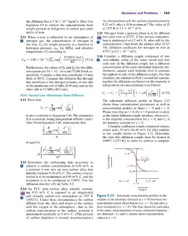
5.12 Show that The schematic diffusion profile in Figure 5.13
B x 2 shows these concentration parameters as well as
C x = expa - b concentration profiles at times t 0 and t 0.
1Dt 4Dt
Please note that at t 0, the x 0 position is taken
is also a solution to Equation 5.4b. The parameter as the initial diffusion couple interface, whereas C 1
B is a constant, being independent of both x and t. is the impurity concentration for x 0, and C 2 is
Hint: From Equation 5.4b, demonstrate that the impurity content for x 0.
B x 2 Consider a diffusion couple composed of pure
0c expa - b d nickel and a 55 wt% Ni-45 wt% Cu alloy (similar
1Dt 4Dt to the couple shown in Figure 5.1). Determine
0t the time this diffusion couple must be heated at
is equal to 1000 C (1273 K) in order to achieve a composi-
B x 2
2 C
0 c expa - b d 1
• 1Dt 4Dt ¶
D 2 t > 0
0x C – C 2
1
5.13 Determine the carburizing time necessary to Concentration 2
achieve a carbon concentration of 0.30 wt% at t = 0
a position 4 mm into an iron–carbon alloy that
initially contains 0.10 wt% C. The surface concen- C 2
tration is to be maintained at 0.90 wt% C, and the
treatment is to be conducted at 1100 C. Use the x < 0 x > 0
diffusion data for g-Fe in Table 5.2. x = 0

5.14 An FCC iron–carbon alloy initially contain- Position
ing 0.55 wt% C is exposed to an oxygen-rich
and virtually carbon-free atmosphere at 1325 K Figure 5.13 Schematic concentration profiles in the
(1052 C). Under these circumstances, the carbon vicinity of the interface (located at x 0) between two
diffuses from the alloy and reacts at the surface semi-infinite metal alloys before (i.e., t 0) and after a
with the oxygen in the atmosphere—that is, the heat treatment (i.e., t 0). The base metal for each alloy
carbon concentration at the surface position is is the same; concentrations of some elemental impurity
maintained essentially at 0 wt% C. (This process are different—C 1 and C 2 denote these concentration
of carbon depletion is termed decarburization.) values at t 0.