Page 188 - Mathematical Models and Algorithms for Power System Optimization

Discrete Optimization for Reactive Power Planning 179
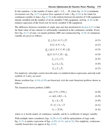
In this equation, i is the number of states, and i¼1,2,…, M, where Eq. (6.16) is minimum
investment cost, Eq. (6.17) is power flow equation of state i, Eq. (6.18) is the limits for
continuous variable of state i, Eq. (6.19) is the relation between the number of VAR equipment
already installed and the number of newly installed VAR equipment, and Eq. (6.20) is the
relation expression of the fixed cost for newly installed VAR equipment.

The difference between constraint of single state and that mentioned in Section 6.5.2 is that
the limit value of line current I is additionally considered in the continuous variable. Power
flow Eq. (6.17) of state i in master problem (MP) and construction Eq. (6.18) of continuous
variable are given as follows:

ð
P P j U, θ, TÞ P j (6.21)
j
P j U, θ, Tð Þ ¼ P js (6.22)
Q Q j U, θ, T, C, RÞ Q (6.23)
ð
j j
ð
Q j U, θ, T, C, RÞ ¼ Q js (6.24)
(6.25)
U U j U j
j
(6.26)
I I kj I kj
kj
(6.27)
T T j T j
j
For simplicity, subscript i used to describe state-i is omitted in these expressions, and only node
symbols of k and j are used.

Master problem Eqs. (6.16)–(6.20) are linearized, with the main linearized problem shown as
follows:
The linearized master problem (LMP):
t t
ð
min C Y C + D W C Þ (6.28)
s:t: A i X i + B i Y i ¼ b i (6.29)
X X i X i (6.30)
i
0 Y i Y C Y (6.31)

Y C Y W C (6.32)
where A i is Jacobi matrix of continuous variable, and B i is coefficient of integer variable.

With multiple states considered, Eqs. (6.28)–(6.32) will be optimization of large scale.
Eq. (6.33) is matrix expression of Eqs. (6.29), (6.31), and (6.32). For simplicity, continuous
variable bound does not appear in Eq. (6.34).