Page 192 - Mathematical Models and Algorithms for Power System Optimization

Discrete Optimization for Reactive Power Planning 183
k k+1
Step 5: The convergence of this procedure is checked, that is, whether |Z Z | meets
convergence conditions. If all variables converge, that is, all subproblems converge, then
the solution algorithm is terminated. The convergence of all the subproblems means that a
solution for nonlinear problem MP has been obtained. Otherwise, k k +1 and
linearize again, then move to Step 2.

6.4.3.2 Decomposition and coordination within main procedure
This is a key procedure for multistate VAR planning problem. As previously mentioned,
linearized subproblem LSP in this section has no objective function, so that it is not applicable
to take objective function of ordinary decomposition and coordination procedure as the
function of coordination variable. Appendix A shows infeasibility and feasibility of a single
state calculated in simplex tableau form.

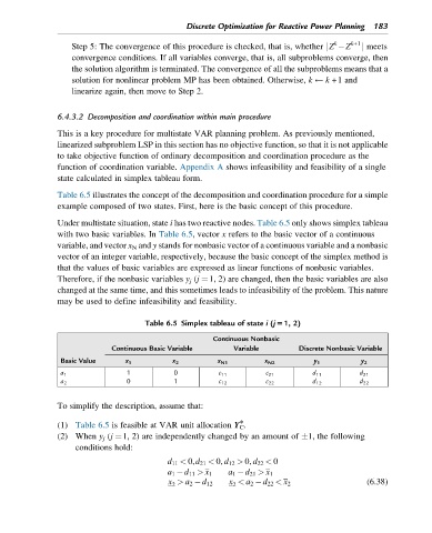
Table 6.5 illustrates the concept of the decomposition and coordination procedure for a simple
example composed of two states. First, here is the basic concept of this procedure.
Under multistate situation, state i has two reactive nodes. Table 6.5 only shows simplex tableau
with two basic variables. In Table 6.5, vector x refers to the basic vector of a continuous
variable, and vector x N and y stands for nonbasic vector of a continuous variable and a nonbasic
vector of an integer variable, respectively, because the basic concept of the simplex method is
that the values of basic variables are expressed as linear functions of nonbasic variables.
Therefore, if the nonbasic variables y j (j ¼1, 2) are changed, then the basic variables are also
changed at the same time, and this sometimes leads to infeasibility of the problem. This nature
may be used to define infeasibility and feasibility.

Table 6.5 Simplex tableau of state i (j51, 2)
Continuous Nonbasic
Continuous Basic Variable Variable Discrete Nonbasic Variable
Basic Value x 1 x 2 x N1 x N2 y 1 y 2
1 0 c 11 c 21 d 11 d 21
a 1
0 1 c 12 c 22 d 12 d 22
a 2
To simplify the description, assume that:
∗
(1) Table 6.5 is feasible at VAR unit allocation Y C .
(2) When y j (j ¼1, 2) are independently changed by an amount of 1, the following
conditions hold:
d 11 < 0,d 21 < 0, d 12 > 0, d 22 < 0

a 1 d 11 > x 1 a 1 d 21 > x 1
(6.38)
x > a 2 d 12 x < a 2 d 22 < x 2
2 2