Page 189 - Mathematical Models and Algorithms for Power System Optimization

180 Chapter 6

A 1 B 1 X 1 = b 1
E –E Y 1 £ 0
B X = b
A 2 2 2 2
E –E Y 2 £ 0
... ... ...
ð6:33Þ
A N B N X N = b N
E –E Y N £ 0
–
E –[Y] Y c £ 0
W c

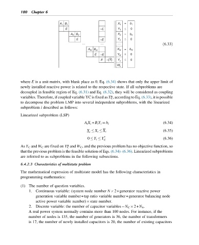
where E is a unit matrix, with blank place as 0. Eq. (6.34) shows that only the upper limit of
newly installed reactive power is related to the respective state. If all subproblems are
decoupled in feasible region of Eq. (6.31) and Eq. (6.32), they will be considered as coupling
variables. Therefore, if coupled variable YC is fixed as Y C ∗, according to Eq. (6.33), it is possible
to decompose the problem LMP into several independent subproblems, with the linearized
subproblem i described as follows:
Linearized subproblem (LSP)

(6.34)
A i X i + B i Y i ¼ b i
X X i X i (6.35)
i
0 Y i Y ∗ (6.36)
C
As Y C and W C are fixed on Y C ∗ and W C , and the previous problem has no objective function, so
that the previous problem is the feasible solution of Eqs. (6.34)–(6.36). Linearized subproblems
are referred to as subproblems in the following subsections.
6.4.2.3 Characteristics of multistate problem

The mathematical expression of multistate model has the following characteristics in
programming mathematics:
(1) The number of question variables.
1. Continuous variable: (system node number N 2+generator reactive power
generation variable number+tap ratio variable number+generator balancing node
active power variable number) state number.
2. Discrete variable: the number of capacitor variables¼N C 2+N E .
A real power system normally contains more than 100 nodes. For instance, if the
number of nodes is 135, the number of generators is 36, the number of transformers
is 17, the number of newly installed capacitors is 20, the number of existing capacitors