Page 198 - Mathematical Models and Algorithms for Power System Optimization

Discrete Optimization for Reactive Power Planning 189

Results of Case 2 are shown in Tables 6.10 and 6.11. Table 6.10 shows integer solutions of
the decomposition and coordination algorithm, whereas Table 6.11 shows the integer
solutions by independent solution method. Similarly, the values in “sum of setting” column in
Table 6.10 are larger than that in Table 6.11. However, the values in “Y C ” column are smaller
than that in Table 6.11, that is, installation cost is smaller by decomposition and coordination
algorithm.
The results of Case 1 show that results of the algorithm proposed is better than independent
solution method in the number of newly installed nodes, as well as the number and cost of newly
installed VAR nodes. The results of Case 2 show that the algorithm proposed obtains a better
solution in the number and cost of newly installed VAR nodes, even if the same number of
newly installed VAR nodes is selected.

To further explain the coordination procedure, Table 6.12 shows the detailed process of total
infeasibility reduction in the first iteration of Case 1:

(1) With integer constraint conditions relaxed, each state will be separately solved by LP. On
this basis, integer solutions of each state will be rounded off, and the maximum value of
integers under each state will be taken as the initial integer solution.
(2) Under initial integer constraint, MILP algorithm in Section 6.3 will be used to solve all
states. At the moment, States 2, 4, and 5 are found infeasible, leading to a total infeasibility
of 0.336.
(3) Coordinate each state: Calculate the infeasibility q ij of each infeasible state, then calculate
total infeasibility q j . According to q j , node 75 is the node that can minimize the infeasible
q ij ; set new VAR unit at the node; repeat the previous procedure, until all states are
feasible, that is, total infeasibility is 0.
(4) Improvement of integer solution: Select a pair of nonzero integers, and add one of the
integers by 1 and reduce another by 1, so as to reduce the fixed costs (Table 6.13).

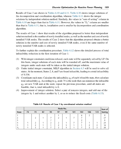
Table 6.8 Results of Case 1 by coordinated solution method
Node No.
Sum of
State 74 75 82 95 97 99 101 102 106 123 Setting

1 1 6 2 9
2 2 1 7 2 1 7 7 27
3 7 2 9
4 1 2 1 2 2 1 7 7 1 1 25
5 1 2 1 1 2 3 1 1 2 2 16
1 2 1 7 2 3 1 7 2 2 28
Y C