
Page 223 - Mathematical Models and Algorithms for Power System Optimization
P. 223
214 Chapter 6
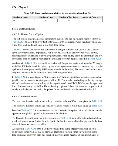
Table 6.26 Basic calculation conditions for the algorithm based on GA
Number of Nodes Number of Lines Number of Tap Ratios Number of Capacitors
38 12 27 7
6.6.5 Implementation
6.6.5.1 38-node Practical System
The test system used is an actual distribution system, and the calculation scale is shown in
Table 6.26. The algorithm is verified by two cases with identical network structures where Case
1 is a low-load mode and Case 2 is a high-load mode.
Table 6.27 shows the calculation conditions of integer variables for Cases 1 and 2 based
upon the computational experience. For the actual system of the previous scale, the GA
breeding can be controlled to about 50 generations, each having about 10 offsprings, and GA
operations shall be carried out under the guidance of expert rules as stated in Section 6.6.4.
As shown in Table 6.27, there are 18 tap ratios and 7 capacitor banks with a total of 25 integer
variables. INI is the condition given by the actual system operators (or alternatively, take the
optimal solutions generated by MILP method as the initial value). For the sake of saving space,
only the stochastic initial solutions INI1–INI3 are given here.
In Table 6.27, the same figure in “Interconnection” indicates that there are interconnected or
parallellinesbetweenthetwointegervariables;“UH”meanstheratedvoltageat thehighvoltage
side of transformer and rated voltage at the capacitor node; and “BOUND” means the upper and
lower limits of integer variables. If the planning engineer fails to determine the upper limit of
newly installed capacitor banks, the power factor at this node may be considered as 1.0.
6.6.5.2 Numerical Results
The objective function values and voltage violation values of Case 1 are given in Table 6.28.
The objective function values and voltage violation values of Case 2 are given in Table 6.29.
Based on Table 6.27, GA operations are executed to make the optimization calculation, and the
approximated global optimal solution would be obtained.
To illustrate the multiplicity of integer solutions, Table 6.30 shows the detailed calculation
results of integer variables for Case 2. Due to the limited space, this table gives only the final
nine solutions for integer variables.
As shown in Table 6.30, SO6–SO9 have obtained the same objective function in spite
of different initial values, that is, there are identical objective function values for these
four solutions. However, only one solution may be chosen because of the multiplicity of