
Page 133 - Mathematical Techniques of Fractional Order Systems
P. 133
Exact Solution of Linear Fractional Distributed Order Systems Chapter | 4 121
Theorem 2 reveals an identity between two expressions (4.83) and (4.84) as
stated in the following Remark.
Remark 2: : The following identity holds true for all λ; t . 0
ð t λτ21 ð 1N
ð
ð t2τÞ ð ð λ 1 1Þτ 2 tÞ τ λ r 1 1Þ 2rt
e dτ 5 2 e dr ð4:94Þ
2 2
ð
0 Γλτ 1 1Þ 0 rλ π 1 rr112λlnrð Þ
4.4 NUMERICAL EXAMPLES
In this section, four examples are presented to evaluate the obtained solutions
of distributed order differential Eqs. (4.17) and (4.82) for different coeffi-
cients and weight functions.
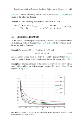
Example 1: Assume x 0ðÞ 5 1. Solutions of (4.82) with
λA 12; 10; 8; 6; 4g ð4:95Þ
f
and the unitary weight function w αðÞ 5 1 ðαA 0; 1Þ are plotted in Fig. 4.1.
½
As it is expected, decay in solutions is more intense for greater values of λ.
Example 2: The first elements of the solutions of (4.17) with utðÞ 5 HtðÞ,a
zero initial condition and different matrix pairs ðA; BÞ given in Table 4.2 are
depicted in Fig. 4.2.
1
λ = 12
0.9
0.8 λ = 10
0.7 λ = 8
0.6
λ = 6
0.5
λ = 4
0.4
0.3
0.2
0.1
0
0 0.1 0.2 0.3 0.4 0.5 0.6 0.7 0.8
t
FIGURE 4.1 Solution of (4.82) with x 0ðÞ 5 1 and the weight function w αðÞ 5 1;αA 0; 1 for
½
different values of λ given by (4.95).