
Page 136 - Mathematical Techniques of Fractional Order Systems
P. 136
124 Mathematical Techniques of Fractional Order Systems
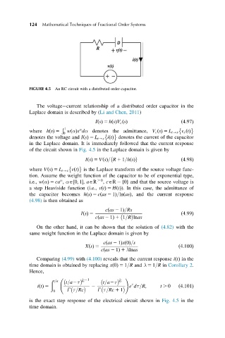
FIGURE 4.5 An RC circuit with a distributed order capacitor.
The voltage current relationship of a distributed order capacitor in the
Laplace domain is described by (Li and Chen, 2011)
IsðÞ 5 hsðÞV c sðÞ ð4:97Þ
α
where hsðÞ 5 Ð 1 w αðÞs dα denotes the admittance, V c sðÞ 5 L t-s v c tðÞ
0
denotes the voltage and IsðÞ 5 L t-s itðÞ denotes the current of the capacitor
in the Laplace domain. It is immediately followed that the current response
of the circuit shown in Fig. 4.5 in the Laplace domain is given by
IsðÞ 5 VsðÞ= R 1 1=hsðÞ ð4:98Þ
where VsðÞ 5 L t-s vtðÞ is the Laplace transform of the source voltage func-
tion. Assume the weight function of the capacitor to be of exponential type,
α . 0
i.e., w αðÞ 5 ca , αA 0; 1, aAR , cAR 2 0fg and that the source voltage is
½
a step Heaviside function (i.e., vtðÞ 5 HtðÞ). In this case, the admittance of
the capacitor becomes hsðÞ 5 cas 2 1Þ=ln asðÞ, and the current response
ð
(4.98) is then obtained as
cas 2 1Þ=Rs
ð
IsðÞ 5 ð4:99Þ
cas 2 1Þ 1 1=R lnas
ð
On the other hand, it can be shown that the solution of (4.82) with the
same weight function in the Laplace domain is given by
cas 2 1Þx 0ðÞ=s
ð
XsðÞ 5 ð4:100Þ
cas 2 1Þ 1 λlnas
ð
Comparing (4.99) with (4.100) reveals that the current response itðÞ in the
time domain is obtained by replacing x 0ðÞ 5 1=R and λ 5 1=R in Corollary 2.
Hence,
τ τ !
ð t=a t=a2τ Rc 21 t=a2τ Rc
τ
itðÞ 5 2 e dτ=R; t . 0 ð4:101Þ
Γτ=Rc Γτ=Rc 1 1
0
is the exact step response of the electrical circuit shown in Fig. 4.5 in the
time domain.