Page 139 - Mathematical Techniques of Fractional Order Systems

Exact Solution of Linear Fractional Distributed Order Systems Chapter | 4 127

6

4

2

Im 0

–2

–4

–6
–8 –6 –4 –2 0 2 4 6 8
Re
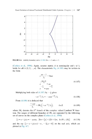
FIGURE 4.6 stability boundary curve (4.106) for c 5 1 and a 5 1.

(Corless et al., 1996). Again, assume matrix A is nonsingular and c 6¼ λ i
holds for all iA 1; 2;...; ng. The characteristic Eq. (4.105) may be written in
f
the form
as 2 1
c 5 lnas
λ i
ð as21Þ
c ð4:107Þ
λ i
e 5 as
c as
2 2c
λ i λ i
e 5 ase
Multiplying both sides of (4.107) by 2 c gives
λ i
2 c 2c as
2ce λ i=λ i 52 case λ i =λ i ð4:108Þ
From (4.108) it is deduced that
2 cas 2 c
5 lW k 2ce λ i=λ i ; kAZ ð4:109Þ
λ i
where lW k denotes the k th branch of the complex valued Lambert W func-
tion. The ranges of different branches of lW k are separated by the following
set of curves on the complex plane (Corless et al., 1996)

s 5 x 1 jyjx 52 ycoty; 2kπ , y , 2k 1 1Þπ; kAN , 0fg ð4:110Þ
ð

and the ray s 5 x 1 jyjxA 2N; 2 1Š; y 5 0 on the real axis, which are
ð
plotted in Fig. 4.7.