Page 138 - Mathematical Techniques of Fractional Order Systems

126 Mathematical Techniques of Fractional Order Systems

matrix A by λ i where iA 1; 2;...; ng. This allows one to write Eq. (4.102) in
f
the following form
W 2lnsÞ 5 λ i ; i 5 1; 2;...; n ð4:103Þ
ð
α
Assuming w αðÞ 5 ca , αA 0; 1Š, aAR . 0 , and cAR 2 0fg would result in
½
the following characteristic equation
ð 1
α
c ðasÞ dα 5 λ i ; i 5 1; 2; ...; n ð4:104Þ
0
from (4.103). In the following discussion, we restrict ourselves to the princi-
pal branch of the complex logarithm function (4.5) since a physical signifi-
cance is only associated with its first Riemann sheet (Jiao et al., 2012,p.
12). If A is singular, then system (4.17) is clearly unstable from (4.104) as
the root s 5 0 is derived for the zero eigenvalue. Also, s 5 1=a satisfies
(4.104) if and only if c 5 λ i holds for some iA 1; 2;...; nf g which also indi-
cates another unstable case of the system. Therefore, assume matrix A is
nonsingular and c 6¼ λ i holds for all iA 1; 2;...; nf g. Based on this assumption,
Eq. (4.104) could be written in the following form
as 2 1
c 5 λ i ; i 5 1; 2;...; n ð4:105Þ
lnas
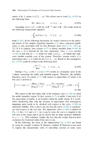
Setting s 5 jω, ωA 0; 1 NÞ in (4.105) results in a boundary curve in the
ð
λ-plane, separating the stable and unstable regions. Therefore, the stability
boundary curve of system (4.17) with respect to eigenvalues of matrix A in
this case is derived as
2 4lnaω 1 2πaω 2π 1 4aωlnaω

s 5 x 6 jyjx 5 c ; y 5 c ; ωAð0; 1 NÞ
2
4lnaωÞ 1 π 2 4lnaωÞ 1 π 2
2
ð
ð
ð4:106Þ
The region on the left (right) side of the boundary curve (4.106) is called
the stable (unstable) region. In fact, system (4.17) is stable, if and only if all
the eigenvalues of matrix A are located within the stable region. It is worth-
while mentioning that, only the location of eigenvalues with nonnegative
imaginary parts needs to be checked with respect to the curve (4.106) to
determine stability. This is due to the fact that the curve (4.106) is symmetri-
cal with respect to the real axis. The parametric curve (4.106) is plotted in
Fig. 4.6 for c 5 1 and a 5 1. As it can be seen, the curve is tangent to the
real axis at the origin and it can be shown that its slope increases infinitely
as ω- 1 N. This somehow implies the fact that the weight function here
comprises the fractional orders from zero to one.
In the following, the roots of the characteristic Eq. (4.105) are found
by using the complex Lambert W function. Lambert W function is also used
to express the characteristic roots of time-delay systems in some cases