
Page 134 - Mathematical Techniques of Fractional Order Systems
P. 134
122 Mathematical Techniques of Fractional Order Systems
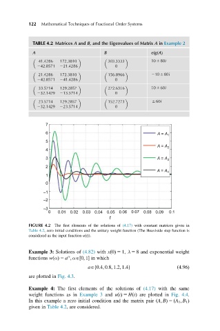
TABLE 4.2 Matrices A and B, and the Eigenvalues of Matrix A in Example 2
A B eig AðÞ
41:4286 172:3810 303:3333 10 6 80i
242:8571 221:4286 0
21:4286 172:3810 156:8966 210 6 80i
242:8571 241:4286 0
33:5714 129:2857 272:6316 10 6 60i
232:1429 213:5714 0
23:5714 129:2857 152:7273 6 60i
232:1429 223:5714 0
7
6 A = A 1
5
A = A 2
4
3 A = A 3
2
A = A 4
1
0
–1
–2
–3
0 0.01 0.02 0.03 0.04 0.05 0.06 0.07 0.08 0.09 0.1
t
FIGURE 4.2 The first elements of the solutions of (4.17) with constant matrices given in
Table 4.2, zero initial conditions and the unitary weight function (The Heaviside step function is
considered as the input function ut ðÞ).
Example 3: Solutions of (4.82) with x 0ðÞ 5 1, λ 5 8 and exponential weight
α
functions w αðÞ 5 a ; αA 0; 1 in which
½
aA 0:4; 0:8; 1:2; 1:4g ð4:96Þ
f
are plotted in Fig. 4.3.
Example 4: The first elements of the solutions of (4.17) with the same
weight functions as in Example 3 and utðÞ 5 HtðÞ are plotted in Fig. 4.4.
In this example a zero initial condition and the matrix pair ðA; BÞ 5 ðA 1 ; B 1 Þ
given in Table 4.2, are considered.