Page 34 - Mathematical Techniques of Fractional Order Systems

24 Mathematical Techniques of Fractional Order Systems

450
400
Osteoclasts C(t) [cells] 300
350
250
200
150
100
50
0 0.1
0.2
0.3 0.4
0.5 3500 4000 4500 5000
0.6
0.7 0.8 2000 2500 3000
0.9 1000 1500
1 0 500
Distance - x ∈ [0,1] Time - t [days]
450
400
Osteoclasts B(t) [cells] 300
350
250
200
150
100
0
0.1 0.2
3500 4000
0.3 0.4 0.5
0.6 2500 3000
0.7 2000
0.8 0.9 1000 1500
Distance - x ∈ [0,1] 1 0 500
Time - t [days]

150
140
Bone mass Z(t) [%] 130 3500 4000
120
110
100
90
80
2000 2500 3000
70 1500
0 0.1 1000
0.2 0.3
0.4 0.5 500
0.6 0.7 0.8 0 Time - t [days]
0.9 1
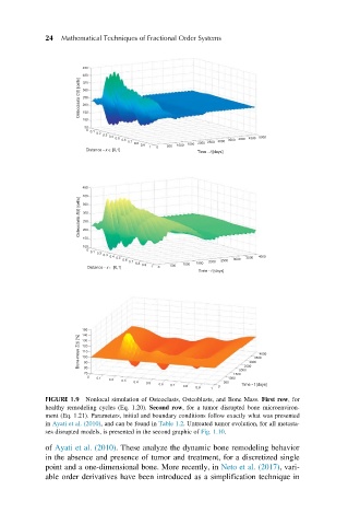
FIGURE 1.9 Nonlocal simulation of Osteoclasts, Osteoblasts, and Bone Mass. First row, for
healthy remodeling cycles (Eq. 1.20). Second row, for a tumor disrupted bone microenviron-
ment (Eq. 1.21). Parameters, initial and boundary conditions follow exactly what was presented
in Ayati et al. (2010), and can be found in Table 1.2. Untreated tumor evolution, for all metasta-
ses disrupted models, is presented in the second graphic of Fig. 1.10.
of Ayati et al. (2010). These analyze the dynamic bone remodeling behavior
in the absence and presence of tumor and treatment, for a discretized single
point and a one-dimensional bone. More recently, in Neto et al. (2017), vari-
able order derivatives have been introduced as a simplification technique in