Page 30 - Mathematical Techniques of Fractional Order Systems

20 Mathematical Techniques of Fractional Order Systems

Monoclonal antibodies and bisphosphonates therapies Monoclonal antibodies
25
Osteoclasts [cells] 20 5 Bisphosphonates
15
10
0
0 500 1000 1500 2000 2500 Monoclonal antibodies 3000
Osteoblasts [cells] 600 Bisphosphonates
800
400
200
0
0 500 1000 1500 2000 2500 3000
110 Monoclonal antibodies
Bone mass [%] 90
100
Bisphosphonates
80
70
60
50
0 500 1000 1500 2000 2500 3000
Time t [days]
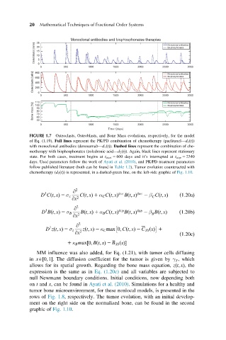
FIGURE 1.7 Osteoclasts, Osteoblasts, and Bone Mass evolutions, respectively, for the model
of Eq. (1.19). Full lines represent the PK/PD combination of chemotherapy (paclitaxel—d 3 ðtÞ)
with monoclonal antibodies (denosumab—d 1 ðtÞ). Dashed lines represent the combination of che-
motherapy with bisphosphonates (zoledronic acid—d 2 ðtÞ). Again, black lines represent stationary
state. For both cases, treatment begins at t start 5 600 days and it’s interrupted at t stop 5 2340
days. Used parameters follow the work of Ayati et al. (2010), and PK/PD treatment parameters
follow published literature (both can be found in Table 1.2). Tumor evolution counteracted with
chemotherapy (d 3 ðtÞ) is represented, in a dashed-green line, on the left-side graphic of Fig. 1.10.

@ 2
1 g CC g BC
D Cðt; xÞ 5 σ c 2 Cðt; xÞ 1 α C Cðt; xÞ Bðt; xÞ 2 β Cðt; xÞ ð1:20aÞ
C
@x
@ 2
1 g CB g BB
D Bðt; xÞ 5 σ B 2 Bðt; xÞ 1 α B Cðt; xÞ Bðt; xÞ 2 β Bðt; xÞ ð1:20bÞ
B
@x
@ 2
1
D zðt; xÞ 5 σ z 2 zðt; xÞ 2 κ C max 0; Cðt; xÞ 2 C SS ðxÞ 1
@x ð1:20cÞ
1 κ B max½0; Bðt; xÞ 2 B SS ðxފ
MM influence was also added, for Eq. (1.21), with tumor cells diffusing
in xA½0; 1Š. The diffusion coefficient for the tumor is given by γ , which
T
allows for its spatial growth. Regarding the bone mass equation, zðt; xÞ, the
expression is the same as in Eq. (1.20c) and all variables are subjected to
null Newmann boundary conditions. Initial conditions, now depending both
on t and x, can be found in Ayati et al. (2010). Simulations for a healthy and
tumor bone microenvironment, for these nonlocal models, is presented in the
rows of Fig. 1.8, respectively. The tumor evolution, with an initial develop-
ment on the right side on the normalized bone, can be found in the second
graphic of Fig. 1.10.