Page 450 - Mathematical Techniques of Fractional Order Systems

Applications of Continuous-time Fractional Order Chapter | 14 435

case. The parameter m was chosen to be m 52 10 in the first case while the
parameter n was chosen to be n 52 5 at the second case. It can be seen that
the system reaches the equilibrium point in less 10 seconds. The initial con-
ditions are x d 5 60 Amp., x q 5 20 Amp. and x a 5 15 rad/sec. It can be seen
that the state variables x a and x q exhibit oscillatory decay while the variable
x d decays without oscillations. Also, the further the value of the variable
from the equilibrium point, the longer the time it takes to stabilize.
Moreover, oscillations from the first case have larger overshoots than in the
second case.
Later on, the authors proposed a synchronization scheme for the same
system (Shen and Zhou, 2016). Consider the system in Eq. (14.68a c) to be
the master system, so the slave system can be written as (Shen and Zhou,
2016):
q
D y d 52 0:875y d 1 y q y a 1 u d ; ð14:70aÞ
q
D y q 52 y q 2 y d y a 1 55y a 1 u q ; ð14:70bÞ
q
D y a 5 4ðy q 2 y a Þ 1 u a ; ð14:70cÞ
where u d , u q , and u a are the feedback controller inputs given by:

2 3 2 3
u d 2x q
5 x d 1 k 2 55 2 γ ðy a 2 x a Þ;
u q
4 5 4 5 ð14:71Þ
0
u a
where k is a real number and was chosen to be equal to either one of the
three cases: 2k q k a , k q , and k a . It was proved that chaos synchronization can
p
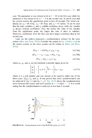
be achieved if jk q j , 1 and jk a j , γ. Fig. 14.14 shows the synchronization
ffiffiffi
errors between the master and slave systems at γ 5 4 and k 52 2. It is worth
noting that the synchronization is achieved in less than 5 seconds.

FIGURE 14.14 Synchronization errors of the BLDCM system at q 5 0:97.