Page 61 - Mathematical Techniques of Fractional Order Systems

Nonlinear Fractional Order Boundary-Value Problems Chapter | 2 51

0

E = 80 CPM
α = 3.9
–50
E = 40

∋
–100

E = 20

–150

0.0 0.5 1.0 1.5 2.0 2.5
h
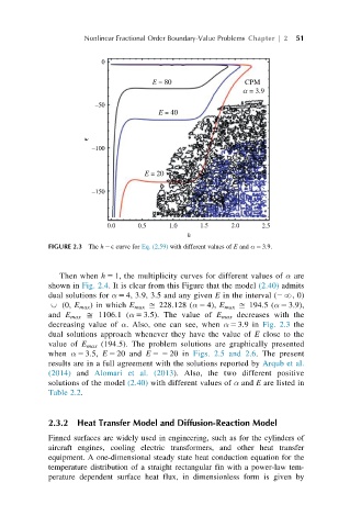
FIGURE 2.3 The h 2 E curve for Eq. (2.59) with different values of E and α 5 3.9.

Then when h 5 1, the multiplicity curves for different values of α are
shown in Fig. 2.4. It is clear from this Figure that the model (2.40) admits
dual solutions for α 5 4, 3.9, 3.5 and any given E in the interval (2N,0)
, (0, E max )inwhich E max D 228.128 (α 5 4), E max D 194.5 (α 5 3.9),
and E max D 1106.1 (α 5 3.5). The value of E max decreases with the
decreasing value of α. Also, one can see, when α 5 3.9 in Fig. 2.3 the
dual solutions approach whenever they have the value of E close to the
value of E max (194.5). The problem solutions are graphically presented
when α 5 3.5, E 5 20 and E 52 20 in Figs. 2.5 and 2.6. The present
results are in a full agreement with the solutions reported by Arqub et al.
(2014) and Alomari et al. (2013). Also, the two different positive
solutions of the model (2.40) with different values of α and E are listed in
Table 2.2.

2.3.2 Heat Transfer Model and Diffusion-Reaction Model

Finned surfaces are widely used in engineering, such as for the cylinders of
aircraft engines, cooling electric transformers, and other heat transfer
equipment. A one-dimensional steady state heat conduction equation for the
temperature distribution of a straight rectangular fin with a power-law tem-
perature dependent surface heat flux, in dimensionless form is given by