Page 62 - Mathematical Techniques of Fractional Order Systems

52 Mathematical Techniques of Fractional Order Systems

300 0
0
–2
–2
–4
200 –4
–6 ∋
= 106.1
E Max –6
–8 E Max = 228.1
100 –10 –8
020 40 60 80 100120
–10
E 0 50 100 150 200 250
E
0
∋
0
–2
–100
–4
α = 3.9
∋
–6
E Max = 194.5 α = 3.5
–200 –8 α = 4
–10
0 50 100 150 200 250
–300 E
–200 –100 0 100 200
E
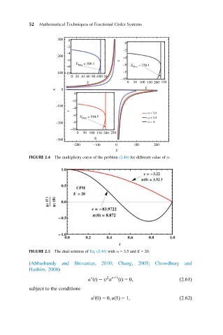
FIGURE 2.4 The multiplicity curve of the problem (2.40) for different value of α.

FIGURE 2.5 The dual solution of Eq. (2.40) with α 5 3.5 and E 5 20.

(Abbasbandy and Shivanian, 2010; Chang, 2005; Chowdhury and
Hashim, 2008)
2 n11
uvðtÞ 2 ψ u ðtÞ 5 0; ð2:61Þ
subject to the conditions

u ð0Þ 5 0; uð1Þ 5 1; ð2:62Þ
0