Page 335 - Matrix Analysis & Applied Linear Algebra

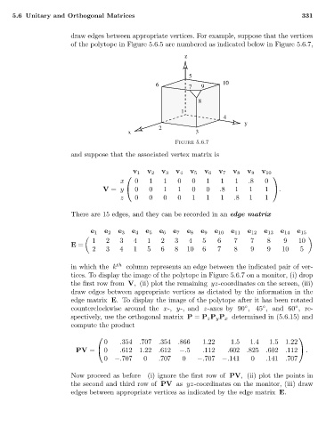
5.6 Unitary and Orthogonal Matrices 331

draw edges between appropriate vertices. For example, suppose that the vertices
of the polytope in Figure 5.6.5 are numbered as indicated below in Figure 5.6.7,
z

5
6 7 9 10

8
1
4
y
2
x 3
Figure 5.6.7
and suppose that the associated vertex matrix is

v 1 v 2 v 3 v 4 v 5 v 6 v 7 v 8 v 9 v 10
 
x 0 1 1 0 0 1 1 1 .8 0
V = y  0 0 1 1 0 0 .8 1 1 1  .
z 0 0 0 0 1 1 1 .8 1 1

There are 15 edges, and they can be recorded in an edge matrix

e 1 e 2 e 3 e 4 e 5 e 6 e 7 e 8 e 9 e 10 e 11 e 12 e 13 e 14 e 15

1 2 3 4 1 2 3 4 5 6 7 7 8 9 10
E =
2 3 4 1 5 6 8 10 6 7 8 9 9 10 5
in which the k th column represents an edge between the indicated pair of ver-
tices. To display the image of the polytope in Figure 5.6.7 on a monitor, (i) drop
the first row from V, (ii) plot the remaining yz-coordinates on the screen, (iii)
draw edges between appropriate vertices as dictated by the information in the
edge matrix E. To display the image of the polytope after it has been rotated
counterclockwise around the x-, y-, and z-axes by 90 , 45 , and 60 , re-
◦
◦
◦
spectively, use the orthogonal matrix P = P z P y P x determined in (5.6.15) and
compute the product
 
0 .354 .707 .354 .866 1.22 1.5 1.4 1.51.22
PV =  0 .612 1.22 .612 −.5 .112 .602 .825 .602 .112  .
0 −.707 0 .707 0 −.707 −.141 0 .141 .707

Now proceed as before—(i) ignore the first row of PV, (ii) plot the points in
the second and third row of PV as yz-coordinates on the monitor, (iii) draw
edges between appropriate vertices as indicated by the edge matrix E.