Page 177 - Mechanical design of microresonators _ modeling and applications

0-07-145538-8_CH04_176_08/30/05

Microbridges: Lumped-Parameter Modeling and Design

176 Chapter Four
3 2 1

l/2

l

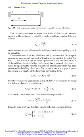
Figure 4.7 Full-length microbridge for torsional resonant frequency calculation.

The lumped-parameter stiffness (the ratio of the torsion moment
applied at the midspan – point 2 – to the resulting angular deforma-
tion) is
4GI t
k t,e = l (4.28)

and this is twice the stiffness of the half-length microbridge [Eq. (4.24)],
as expected.
The distribution function, which is needed to determine the lumped-
parameter mechanical moment of inertia corresponding to point 2 in
Fig. 4.7, and which is dynamically equivalent to the distributed mass
of the full-length microbridge undergoing free torsional vibrations, is
found by applying the method of unknown coefficients which has been
presented for bending vibrations. The torsional angle at a generic point
of abscissa x is sought of the following polynomial form:

ș (x) = a + bx + cx 2 (4.29)
x
The three unknown coefficients in Eq. (4.29) are determined by using
the following boundary conditions:
l
ș (0) = ș (l) =0 ș x( ) = ș x (4.30)
x
x
2
As a result, the distribution function can be expressed as
ș (x) 4x(l í x)
f (x) = x = 2 (4.31)
t
ș
x l
It can be seen that this function satisfies the expected conditions:

0 x =0 and x = l
f (x) = l (4.32)
t
{ 1 x =
2

Downloaded from Digital Engineering Library @ McGraw-Hill (www.digitalengineeringlibrary.com)
Copyright © 2004 The McGraw-Hill Companies. All rights reserved.
Any use is subject to the Terms of Use as given at the website.