Page 327 - Mechanical Engineers' Handbook (Volume 2)

318 Mathematical Models of Dynamic Physical Systems

dx dx dx dT
3
2
a 3 a 2 a 1 ax b 1
0
dt 3 dt 2 dt dt
where the coefficients are unchanged.
For many systems, combining element laws and system relations can best be achieved
by ad hoc procedures. For more complicated systems, formal methods are available for the
orderly combination and reduction of equations. These are the so-called loop method and
node method and correspond to procedures of the same names originally developed in con-
nection with electrical networks. The interested reader should consult Ref. 1.

4.3 State-Variable Form

For systems with multiple inputs and outputs, the I/O model form can become unwieldy. In
addition, important aspects of system behavior can be suppressed in deriving I/O equations.
The ‘‘modern’’ representation of dynamic systems, called the state-variable form, largely
eliminates these problems. A state-variable model is the maximum reduction of the original
element laws and system relations that can be achieved without the loss of any information
concerning the behavior of a system. State-variable models also provide a convenient rep-
resentation for systems with multiple inputs and outputs and for systems analysis using
computer simulation.
State variables are a set of variables x (t), x (t),..., x (t) internal to the system from
2
n
1
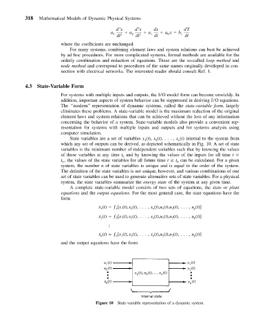
which any set of outputs can be derived, as depicted schematically in Fig. 10. A set of state
variables is the minimum number of independent variables such that by knowing the values
of these variables at any time t and by knowing the values of the inputs for all time t
0
t , the values of the state variables for all future time t t can be calculated. For a given
0
0
system, the number n of state variables is unique and is equal to the order of the system.
The definition of the state variables is not unique, however, and various combinations of one
set of state variables can be used to generate alternative sets of state variables. For a physical
system, the state variables summarize the energy state of the system at any given time.
A complete state-variable model consists of two sets of equations, the state or plant
equations and the output equations. For the most general case, the state equations have the
form
˙ x (t) ƒ[x (t),x (t),..., x (t),u (t),u (t),..., u (t)]
1
2
2
n
p
1
1
1
˙ x (t) ƒ[x (t),x (t),..., x (t),u (t),u (t),..., u (t)]
2
n
2
1
1
2
2
p

˙ x (t) ƒ[x (t),x (t),..., x (t),u (t),u (t),..., u (t)]
p
2
2
n
1
n
1
n
and the output equations have the form
Figure 10 State-variable representation of a dynamic system.