Page 332 - Mechanical Engineers' Handbook (Volume 2)

5 Approaches to Linear Systems Analysis 323

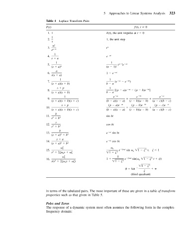
Table 4 Laplace Transform Pairs
F(s) f(t), t 0
1. 1 (t), the unit impulse at t 0
1
2. 1, the unit step
s
n!
3. t n
s n 1
1
4. e at
s a
1 1
e
5. t n 1 at
(s a) n (n 1)!
a
6. 1 e at
s(s a)
1 1
7. (e at e bt )
(s a)(s b) b a
s p 1
8. [(p a)e at (p b)e bt ]
(s a)(s b) b a
1 e at e bt e ct
9.
(s a)(s b)(s c) (b a)(c a) (c b)(a b) (a c)(b c)
s p (p a)e at (p b)e bt (p c)e ct
10.
(s a)(s b)(s c) (b a)(c a) (c b)(a b) (a c)(b c)
b
11. sin bt
2
s b 2
s
12. cos bt
2
s b 2
b
13. e at sin bt
2
(s a) b 2
s a
14. e at cos bt
2
(s a) b 2
2
n n
2
15. e
t n sin 1
t,
1
2 2 2 n
n
s 2
s n 1
2 1
n
2
16. 1 e
t n sin( 1
t )
n
2
2
s(s 2
s ) 1
2
n
n
1
2
tan 1

(third quadrant)
in terms of the tabulated pairs. The most important of these are given in a table of transform
properties such as that given in Table 5.
Poles and Zeros
The response of a dynamic system most often assumes the following form in the complex-
frequency domain: