Page 333 - Mechanical Engineers' Handbook (Volume 2)

324 Mathematical Models of Dynamic Physical Systems

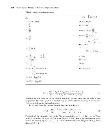
Table 5 Laplace Transform Properties

F(s) f(t)e st dt
f(t) 0
1. aƒ 1 (t) bƒ 2 (t) aF 1 (s) bF 2 (s)
dƒ
2. sF(s) ƒ(0)
dt
d ƒ sF(s) sƒ(0)
dƒ
2
3. 2
dt 2 dt t 0
sF(s) n k
n
n
n
d ƒ k 1 s g k 1
4.
ƒ
k 1
d
dt n
g k 1
dt k 1
t 0
F(s) h(0)

t s s
5. ƒ(t) dt h(0) ƒ(t) dt
0
6. 0, t D t 0
ƒ(t D), t D e sD F(s)
7. e at ƒ(t) F(s a)
8. ƒ
t
a aF(as)
t
9. ƒ(t) x(t )y( ) d F(s) X(s)Y(s)
0
t
y(t )x( ) d
0
10. ƒ( ) lim sF(s)
s→0
11. ƒ(0 ) lim sF(s)
s→
m
N(s) bs b m 1 s m 1 bs b 0
1
m
F(s) (1)
n
D(s) s a n 1 s n 1 as a 0
1
Functions of this form are called rational functions, because these are the ratio of two
polynomials N(s) and D(s). If n m, then F(s)isa proper rational function; if n m, then
F(s)is a strictly proper rational function.
In factored form, the rational function F(s) can be written as
N(s) b (s z )(s z ) (s z )
m
1
2
m
F(s) (2)
D(s) (s p )(s p ) (s p )
n
2
1
The roots of the numerator polynomial N(s) are denoted by z , j 1, 2,..., m. These
j
numbers are called the zeros of F(s), since F(z ) 0. The roots of the denominator poly-
j
nomial are denoted by p ,1,2,..., n. These numbers are called the poles of F(s), since
i
lim F(s) .
s→p i