Page 330 - Mechanical Engineers' Handbook (Volume 2)

5 Approaches to Linear Systems Analysis 321

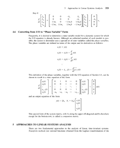
Step 6
0 0 k 1 k 1
ƒ
ƒ
0
k 1
k 1
d ƒ k 2 0 0 0 k 2 ƒ k 2 k 2
dt v m 1 1/m 1 0 1/mb 1/mb v m 1 0 v s
1
1
v 1/m 1/m 1/mb 1/mb v 0
m 2 2 2 2 2 m 2
4.6 Converting from I/O to ‘‘Phase-Variable’’ Form
Frequently, it is desired to determine a state-variable model for a dynamic system for which
the I/O equation is already known. Although an unlimited number of such models is pos-
sible, the easiest to determine uses a special set of state variables called the phase variables.
The phase variables are defined in terms of the output and its derivatives as follows:
x (t) y(t)
1
d
x (t) ˙x (t) y(t)
2
1
dt
d 2
x (t) ˙x (t) y(t)
2
3
dt 2

d n 1
x (t) ˙x n 1 (t) y(t)
n
dt n 1
This definition of the phase variables, together with the I/O equation of Section 4.1, can be
shown to result in a state equation of the form
0 0 1 0 0 1 0 0
x (t)
x (t)
0
1
1
x (t)
0
0
x (t)

2
2
d
dt n 1 (t) 0 0 0 x n 1 (t) u(t)
1
x
x (t) a 0 a 1 a 2 a n 1 x (t) 1
n
n
and an output equation of the form

y(t) [b 0 b b ] x (t)
1
1
m
x (t)
2

x (t)
n
This special form of the system matrix, with 1s along the upper off-diagonal and 0s elsewhere
except for the bottom row, is called a companion matrix.
5 APPROACHES TO LINEAR SYSTEMS ANALYSIS
There are two fundamental approaches to the analysis of linear, time-invariant systems.
Transform methods use rational functions obtained from the Laplace transformation of the