Page 329 - Mechanical Engineers' Handbook (Volume 2)

320 Mathematical Models of Dynamic Physical Systems

4.4 Deriving the ‘‘Natural’’ State Variables—A Procedure
Because the state variables for a system are not unique, there are an unlimited number of
alternative (but equivalent) state-variable models for the system. Since energy is stored only
in generalized system storage elements, however, a natural choice for the state variables is
the set of through and across variables corresponding to the independent T-type and A-type
elements, respectively. This definition is sometimes called the set of natural state variables
for the system.
For linear systems, the following procedure can be used to reduce the set of element
laws and system relations to the natural state-variable model.
Step 1. For each independent T-type storage, write the element law with the derivative
1
of the through variable isolated on the left-hand side, that is, ƒ ˙ L v.
Step 2. For each independent A-type storage, write the element law with the derivative
of the across variable isolated on the left-hand side, that is, ˙v C ƒ.
1
Step 3. Solve the compatibility equations, together with the element laws for the ap-
propriate D-type and multiport elements, to obtain each of the across variables of the inde-
pendent T-type elements in terms of the natural state variables and specified sources.
Step 4. Solve the continuity equations, together with the element laws for the appro-
priate D-type and multiport elements, to obtain the through variables of the A-type elements
in terms of the natural state variables and specified sources.
Step 5. Substitute the results of step 3 into the results of step 1; substitute the results
of step 4 into the results of step 2.
Step 6. Collect terms on the right-hand side and write in vector form.

4.5 Deriving the ‘‘Natural’’ State Variables—An Example
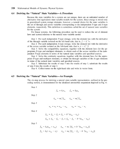
The six-step process for deriving a natural state-variable representation, outlined in the pre-
ceding section, is demonstrated for the idealized automobile suspension depicted in Fig. 6:
Step 1
˙
˙
ƒ k v ƒ k v
k 1 1 k 1 k 2 2 k 2
Step 2
˙ v m ƒ ˙ v m ƒ
1
1
m 1 1 m 1 m 2 2 m 2
Step 3
v v v v v v v
k 1 b m 2 m 1 k 2 m 2 s
Step 4
1
ƒ ƒ ƒ ƒ b (v v )
m 1 k 1 b k 1 m 2 m 1
ƒ ƒ ƒ ƒ ƒ ƒ b (v v )
1
m 2 k 2 k 1 b k 2 k 1 m 2 m 1
Step 5
˙ ƒ k (v v ) ˙ v m [ƒ b (v v )]
1
1
k 1 1 m 2 m 1 m 1 1 k 1 m 2 m 1
˙ ƒ k ( v v ) ˙ v m [ƒ ƒ b (v v )]
1
1
k 2 2 m 2 s m 2 2 k 2 k 1 m 2 m 1