Page 125 - Mechanics of Asphalt Microstructure and Micromechanics

Experimental Methods to Characterize the Heterogeneous Strain F ield 117

Where x j , y j , z j are the center coordinates of the j cross-section; A j is the cross sec-
th
th
tional areas of particle i on the j slice; and H j–1–j is the distance between two adjacent
slices (H j–1–j = z j − z j–1 ).
4.3.6 Computation of Macro Strain
Once the matching particles before and after testing are identified, the translation of the
particles can be calculated from the mass center difference before and after testing,
which was shown in the following equation:
u = X a − X b v = Y a − Y b w = Z a − Z b (4-18)
mc mc mc mc mc mc
Where b represents before testing; a represents after testing. For each of the four
closest particles (i, j, k, l), the displacements u i , u j , u k , u l are in the x direction; v i , v j , v k , v l
are in the y direction; and w i , w j , w k , w l are in the z direction. If the displacement field is
linearly interpolated in a tetrahedron, the displacement can be expressed as the follow-
ing equation.
u = a + a x a y a z
+
+
0 1 2 3
+
+
v = b + b x b y b z (4-19)
0 1 2 3
+
w = c + c x c y c z
+
0 1 2 3
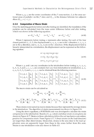
Where x, y, and z are any coordinates in the tetrahedron before testing; a 0 , a 1 , a 2 , a 3 ,
b 0 , b 1 , b 2 , b 3 and c 0 , c 1 , c 2 , c 3 are constants but vary from tetrahedron to tetrahedron. a 0 , a 1 ,
a 2 , a 3 , b 0 , b 1 , b 2 , b 3 and c 0 , c 1 , c 2 , c 3 can be obtained from the following matrices.
xyz ⎤ ⎧ ⎫
xyz ⎤ ⎧ ⎫
⎡ 1,, , a ⎧ ⎧ u ⎫ 1,, ,xyz ⎤ ⎧ ⎫ ⎧v ⎫ 1,, , c ⎧ w ⎫
⎡
⎡
b
⎢ i i i ⎥ ⎪ ⎪ ⎪ i ⎪ ⎢ i i i ⎥ ⎪ ⎪ ⎪ i ⎪ ⎢ i i i ⎥ ⎪ ⎪ ⎪ i ⎪
0
0 0
0
⎢ ⎢ 1,, j , j ⎥⎪ ⎪ ⎪ u j ⎪ ⎢ 1,,xyz j ⎥⎪ ⎪ ⎪ v j ⎪ ⎢ 1, x yz, j , j ⎥ c ⎪ ⎪ ⎪ w j ⎪
xyz
,
a
b
1
j j
1
1
j
j
j
⎬
⎢ ⎥ ⎨ ⎬ = ⎨ ⎬ ⎢ ⎥ ⎨ ⎬ = ⎨ ⎬ ⎢ ⎥ ⎨ ⎬ = ⎨ ⎬ (4-20)
b
,
a
c
,
⎪
⎪
⎢ 1,xyz k ⎥ ⎪ ⎪ ⎪ u k ⎪ ⎢ 1,xy z z k ⎥ ⎪ ⎪ ⎪ k ⎢ , 1 xyz k ⎥ ⎪ ⎪ ⎪ w k ⎪
v
,
,
,
,
k
k
k
2
2
k
k
2
k
⎢ 1,, , ⎥ ⎪ ⎪ ⎪ u ⎪ ⎢ 1,, ⎥ ⎪ ⎪ ⎪ v ⎪ ⎢ 1 ,, , ⎥ ⎪ ⎪ ⎪ w ⎪
c
a
b
xyz
xyz ,
xyz
3
3
3
⎣ l l l ⎦⎩ ⎭ ⎩ l ⎭ ⎣ l l l ⎦⎩ ⎭ ⎩ l ⎭ ⎣ l l l ⎦⎩ ⎭ ⎩ l ⎭
The macro strain can be calculated as:
u ∂ v ∂ ∂ w
ε = = a ε = = b ε = = c
x x ∂ 1 y y ∂ 2 z z ∂ 3
w
ε = 1 ⎛ v ∂ + u ∂ ⎞ = b + a 2 ε = 1 ⎛ ⎛ ⎜ u ∂ + ∂ w⎞ ⎟ = a 3 + c 1 ε = 1 ⎛ ∂v + ∂ ⎞ = b 3 + c 2 (4-21)
1
xy 2 ⎜ ⎝ x ∂ y ∂ ⎠ ⎟ 2 xz 2 ⎝ z ∂ x ∂ ⎠ 2 yz 2 ⎜ ⎝ ∂z ∂ ⎠ ⎟ 2
y

These strains were named as macro-strains because they represent the average strains
in the tetrahedron. The algorithm of strain measurement was shown in Figure 4.16.
Using the above equations, a FORTRAN code was developed to calculate the strain
components in the tetrahedron. Results of x, y, z strain and shear strain on one plane are
shown in Figure 4.17. Strains in these calculations follow the soil mechanics convention:
positive for compressive strain. From Figure 4.17, Y direct strains (in the load direction)
are larger than other direct strains. Meanwhile, strains in the area close to the load ap-
plication zone are apparently larger than those in the zones farther from this zone.
Strains in one tetrahedron were also shown in Table 4.5.