Page 151 - Mechanics of Asphalt Microstructure and Micromechanics

Mixture T heor y and Micromechanics Applications 143

In other words, the effective modulus is:
− N
L = L + ∑ c L −( L A (5-86)
)
0 i=1 i i 0 i
Please note that the above formulation does not make assumptions regarding the
shape of the inclusions. It does not address the misfit of the strain fields between the
matrix and the inclusions. Following the similar philosophy, equation for the compli-
ance tensor can be derived:
− N
M = M + ∑ c M −( M B ) (5-87)
0 i=1 i i 0 i
− −
σ = B σ (5-88)
i i
B i is the stress concentration tensor.
It should be noted that the above formulations are based on relationships with the
average strain or stress of the entire composite. Formulations can be derived using the
relationship between strains/stresses of inhomogeneities with the average strains/
stresses in the matrix.
− −
ε = G ε σ = H σ (5-89a, b)
i i 0 i i 0
The above formulations and the Eshelby tensor form the basis of effective moduli
computations of the Eshelby method, the Mori-Tanaka method, the Self-consistent meth-
od and the Differential Area method. These methods vary with the choice of the refer-
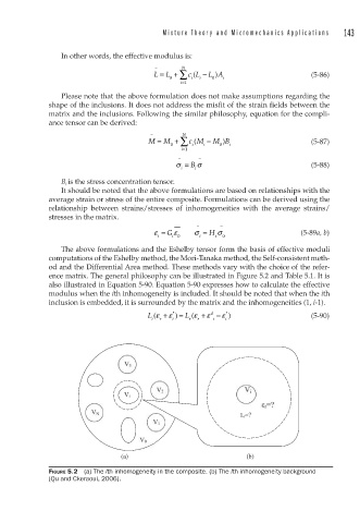
ence matrix. The general philosophy can be illustrated in Figure 5.2 and Table 5.1. It is
also illustrated in Equation 5-90. Equation 5-90 expresses how to calculate the effective
modulus when the ith inhomogeneity is included. It should be noted that when the ith
inclusion is embedded, it is surrounded by the matrix and the inhomogeneities (1, i-1).
L (ε + ε * ) = L (ε + ε − ε * ) (5-90)
d
i r i r r i i

V 3

V 2 V i
V i
r=?
V N
L r=?
V 1

V 0
(a) (b)

FIGURE 5.2 (a) The ith inhomogeneity in the composite. (b) The ith inhomogeneity background
(Qu and Ckeraoui, 2006).