Page 28 - Mechanics of Asphalt Microstructure and Micromechanics

Introduction and Fundamentals for Mathematics and Continuum Mechanics 21

Where dV is the volume of the infinitesimal tetrahedron.
dS
Dividing both sides of the above equation by dS, and considering n = i and
dV i dS
= 0 when dS approaches zero, one obtains:
dS
t n () = t e () 1 n + t e ( 2 ) n + t e () n (1-102)
3
i i 1 i 2 i 3
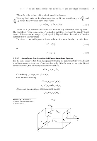
Where i = 1,2,3, therefore the above equation actually represents three equations.
The nine stress vector components t i as a set of quantities represent the Cauchy stress
(e j )
tensors. It is represented as s ij = t i (i = 1,3; j = 1,3). Figure 1.6 is an illustration of the nine
e j
components of a stress tensor.
The stress vector on the plane with normal direction n can then be generalized as:
t i n () = σ ji n j (1-103)
or

n σ
t n () =• (1-104)
1.6.3.3 Stress Tensor Transformation in Different Coordinate Systems
For the same stress vector, it can be represented using the components in two different
coordinate systems, the e i and e i systems. Logically (it is the same vector but different
representations), the following relationship will hold.
n ()
t n () = t e = t n ( ) e
i i r r
(n) (n)
Considering t i = s ji n j and t r = s rs n s
One has the following:

t n () = σ n e = σ n e
ji j i rs r s
n = T n and e = T e
r rl l s sk k
After some manipulations of the summed indices:
σ ne = T T σ n e

ij j i rl sk rs l k

FIGURE 1.6 Schematic x 3
diagram for components of
stress tensor.
σ
33

σ σ 32 σ 23
31
σ σ
13 22
σ σ x 2
σ 12 21
11

x 1