Page 300 - Mechanics of Asphalt Microstructure and Micromechanics

292 Ch a p t e r N i n e

m Maxwell Kelvin
1
section section
Cm
n Maxwell m
section 1
Km Kk
n k
Kelvin
Ck Kk
n n
section f k
Cm
k Km k
Ck
k
m m
2 2

Ball-Ball Ball-Wall Ball-Ball Ball-Wall
Normal Direction Shear Direction

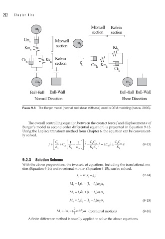
FIGURE 9.6 The Burger model (normal and shear stiffness) used in DEM modeling (Itasca, 2005).

The overall controlling equation between the contact force f and displacement u of
Burger’s model (a second-order differential equation) is presented in Equation 9-13.
Using the Laplace transform method from Chapter 6, the equation can be convenient-
ly solved.
⎡ C ⎛ 1 ⎞ ⎤ · CC CC
·
f + ⎢ k + C m ⎜ + 1 ⎟ f ⎥ + k m ¨ f f =± C u ± k m u ¨ (9-13)
⎣ ⎢ K k ⎝ K k K ⎠ ⎥ KK m m K k
m ⎦
k

9.2.3 Solution Scheme
With the above preparations, the two sets of equations, including the translational mo-
tion (Equation 9-14) and rotational motion (Equation 9-15), can be solved.
F = m x −( ¨ g ) (9-14)
i i i
·
M = ω + ( I − I ω ω)
I
1 1 1 3 2 3 2
·
M = ω + ( I − I ω ω
)
I
2 2 2 1 3 1 3
·
M = ω + ( I − I ω ω) (9-15)
I
3 3 3 2 1 2 1
·
M = Iω = ( 2 mR ω (rotational motion) (9-16)
2
)
i i i
5
A finite difference method is usually applied to solve the above equations.