Page 303 - Mechanics of Asphalt Microstructure and Micromechanics

Applications of Discrete Element Method 295

X-ray
One pixel
(2D)

(a) Geomaterial
(c) Particle cross-section in the
layer

(d) Small balls are used to replace
(b) One layer from the pixels in composing the particles
specimen
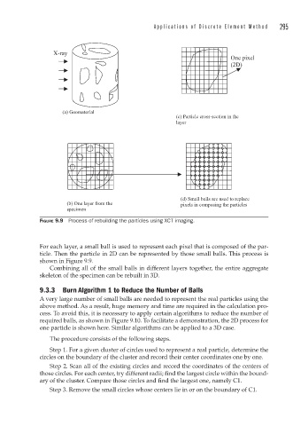
FIGURE 9.9 Process of rebuilding the particles using XCT imaging.

For each layer, a small ball is used to represent each pixel that is composed of the par-
ticle. Then the particle in 2D can be represented by those small balls. This process is
shown in Figure 9.9.
Combining all of the small balls in different layers together, the entire aggregate
skeleton of the specimen can be rebuilt in 3D.

9.3.3 Burn Algorithm 1 to Reduce the Number of Balls
A very large number of small balls are needed to represent the real particles using the
above method. As a result, huge memory and time are required in the calculation pro-
cess. To avoid this, it is necessary to apply certain algorithms to reduce the number of
required balls, as shown in Figure 9.10. To facilitate a demonstration, the 2D process for
one particle is shown here. Similar algorithms can be applied to a 3D case.
The procedure consists of the following steps.

Step 1. For a given cluster of circles used to represent a real particle, determine the
circles on the boundary of the cluster and record their center coordinates one by one.
Step 2. Scan all of the existing circles and record the coordinates of the centers of
those circles. For each center, try different radii; find the largest circle within the bound-
ary of the cluster. Compare those circles and find the largest one, namely C1.
Step 3. Remove the small circles whose centers lie in or on the boundary of C1.