Page 478 - Mechanics of Asphalt Microstructure and Micromechanics

APPENDIX3

Isotropic Elastostatics Fundamental Solution

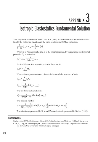
This appendix is abstracted from Gaul et al (2003). It documents the fundamental solu-
tion to the following equation as the basis solution for BEM applications.
1 * * 1 ξ δ
−
12ν u ik kj + u ij kk = − δ x(, ) ij
μ
,
,
Where n is Poisson’s ratio and m is the shear modulus. By introducing the tensorial
potential G ij , one obtains:
u = G − 1 G
*
ij ij mm ( −ν im jm
,
,
21 )
For the 3D case, the tensorial potential function is:
Gr() = 1 rδ
ij 8πμ ij
Where r is the position vector. Some of the useful derivatives include:

G = 1 δ r
ij m 8πμ ij m
,
,
G = 1 δδ − rr )
(
,
ij mn 8πμ r ij mn , m n
,
The fundamental solution is:
1
34νδ
u = (( − ) + rr )
*
ij 16πμ ( − r ) ν ij i ,, j
1
The traction field is:
1 ⎛ r ∂ ⎞
t = (( − ) + 3 rr ) + 12νν)(rn − r n j ⎟
( −
12νδ
*
)
ij π ( − r ) ν 2 ⎜ ⎝ ij i ,, j n ∂ , ji ,i ⎠
81
The solution represented in X, Y and Z coordinates is presented in Becker (1992).
References
Becker, A.A. (1992). The Boundary Element Method in Engineering. McGraw-Hill Book Company.
Gaul, L., Kogl, M. and Wagner, M. (2003). Boundary Element Methods for Engineers and Scientists-
An Introductory Course with Advanced Topics, Springer.

470