Page 178 - MODELING OF ASPHALT CONCRETE

156 Cha pte r S i x

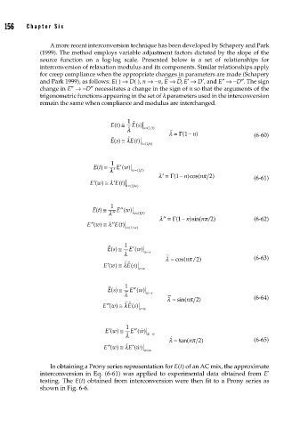
A more recent interconversion technique has been developed by Schapery and Park
(1999). The method employs variable adjustment factors dictated by the slope of the
source function on a log-log scale. Presented below is a set of relationships for
interconversion of relaxation modulus and its components. Similar relationships apply
for creep compliance when the appropriate changes in parameters are made (Schapery
∼
∼
and Park 1999), as follows: E( ) → D( ), n → −n, E → D, E′ → D′, and E″ → −D″. The sign
change in E″ → −D″ necessitates a change in the sign of n so that the arguments of the
trigonometric functions appearing in the set of l parameters used in the interconversion
remain the same when compliance and modulus are interchanged.

Et() ≅ 1 E s)
(

λ s (/
=
1
t)
n
λ = Γ(1 − ) (6-60)

Es () ≅ λ E t ( )
t (1
=
s)
( ′
Et() ≅ 1 E w)
′ λ w (1 t)
=
λ ′ = Γ(1 − )cos(n n π 2 ) (6-61)
′ Ew() ≅ ′E t( )λ
t =(1 w)
( ′′
Et() ≅ 1 E w)
=
λ ′′ w (1 t) λ ′′ = Γ(1 − )sin(n n π/ ) (6-62)
2
Ew ≅ ′′E t( )λ
′′()
1
= t (/ w)

Es () ≅ 1 E w)
( ′
=
λ ws
2
λ = cos(n π/ ) (6-63)
′ Ew() ≅ E s( )λ
= sw

( ′′
Es () ≅ 1 E w)
=
λ ws λ = sin(n π 2 ) (6-64)
′′()
Ew ≅ E s( )λ
= sw
′ Ew() ≅ 1 E ′′ w() ww
=

λ
λ = tan(n π 2 ) (6-65)

′
′′() λ
Ew ≅ E w()
=

ww
In obtaining a Prony series representation for E(t) of an AC mix, the approximate
*
interconversion in Eq. (6-61) was applied to experimental data obtained from E
testing. The E(t) obtained from interconversion were then fit to a Prony series as
shown in Fig. 6-6.