Page 43 - Modelling in Transport Phenomena A Conceptual Approach

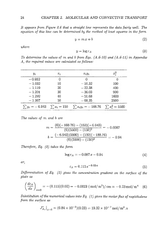
24 CHAPTER 2. MOLECULAR AND CONVECTWE TRANSPORT

It appears from Figure 2.6 that a straight line represents the data fairly well. The
equation of this line can be determined by the method of least squares in the form

y=m~+b (2)

where
y 1OgcA (3)
To determine the values of m and b from Eqs. (A.6-10) and (A.6-11) in Appendix
A, the required values are calculated as follows:

Yi Xi XiYi 23
- 0.932 0 0 0
- 1.032 10 - 10.32 100
- 1.119 20 - 22.38 400
- 1.201 30 - 36.03 900
- 1.292 40 - 51.68 1600
- 1.367 50 - 68.35 2500
vi = - 6.943 = 150 ~iyi = - 188.76 X? = 5500

The values of m and b are

(6)(- 188.76) - (150)(-6.943)
m= = - 0.0087
(6)(5500) - (150)'
(-6.943)(5500) - (150)(- 188.76)
b= = -0.94
(6)(5500) - (150)'

Therefore, Eq. (2) takes the form

Diferentiation of Eq. (5) gives the concentration gradient on the surface of the
plate as
Wz=, (6)
= - (0.115)(0.02) = - 0.0023 ( mol/ m3)/ cm = - 0.23 mol/ m4

Substitution of the numerical values into Eq. (1) gives the molarflax of naphthalene
from the surface as

Jiz = (0.84 x 10-5)(0.23) = 19.32 x 10- mol/ m2. s