Page 278 - Modern Control Systems

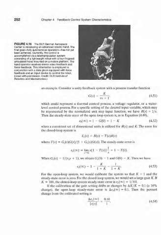
252 Chapter 4 Feedback Control System Characteristics

FIG U R E 4.16 The DLR German Aerospace
Center is developing an advanced robotic hand. The
final goal—fully autonomous operation—has not yet
been acheived. Currently, the control is
accomplished via atelemanipulation system
consisting of a lightweight robot with a four-fingered
articulated hand mounted on a mobile platform. The
hand operator receives stereo video feedback and
force feedback. This information is employed in
conjunction with a data glove equipped with force
feedback and an input device to control the robot.
(Used with permission. Credit: DLR Institute of
Robotics and Mechatronics.)

an example. Consider a unity feedback system with a process transfer function
K
G(s) = (4.51)
TS + 1 ^
which could represent a thermal control process, a voltage regulator, or a water-
level control process. For a specific setting of the desired input variable, which may
be represented by the normalized unit step input function, we have R(s) = l/s.
Then the steady-state error of the open-loop system is, as in Equation (4.49),
^0(00) = 1 - G(0) = \~ K (4.52)

when a consistent set of dimensional units is utilized for R(s) and A'. The error for
the closed-loop system is
E e(s) = R(s) - T(s)R(s)

where T(s) = G c(s)G(s)/(l + G c(s)G(s)). The steady-state error is

e e(oo) = lims{l - T(s)}~ = 1 - T(0).

When G c(s) = 1/(T 1.V + 1), we obtain G c.(0) = 1 and G(0) = K. Then we have
K l
*c(°°) = 1 (4.53)
1 + K 1 + A"
For the open-loop system, we would calibrate the system so that K = 1 and the
steady-state error is zero. For the closed-loop system, we would set a large gain K. If
K = 100, the closed-loop system steady-state error is e c.(oo) = 1/101.
If the calibration of the gain setting drifts or changes by AK/K = 0.1 (a 10%
change), the open-loop steady-state error is A<?„(co) = 0.1. Then the percent
change from the calibrated setting is
Ae ()(oo) 0.10
(4.54)
KOI