Page 230 - Modern Control of DC-Based Power Systems

194 Modern Control of DC-Based Power Systems

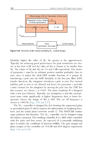
Offline design of K (s) Calculation of duty cycle
Weighting function design K
H-infinity optimisation

V bus
+ e d = Ke

V bus,ref

Measurements Plant: Control signal
generators and loads

Figure 5.55 Overview of the mixed sensitivity H N control design.

Similarly, higher the value of M s , the greater is the aggressiveness.
Typically, for achieving good performance the peak sensitivities are cho-
sen at less than 6 dB and the value of M T is chosen to be smaller than
M s . The values of M s and M T are 4.5 and 3 dB respectively. The choice
of parameter ε must be an arbitrary positive number preferably close to
zero, since it makes the ideal HPF transfer function of S proper by
introducing a pole into the LHP. Similarly, in the low pass filter (LPF)
transfer functions, the integrator introduces a pole at zero. For internal
stability, pole at zero is not allowed and hence the parameter ε provides
a time constant for the integrator by moving the pole into the LHP. For
this scenario, we choose ε as 0.003. The noise sensitivity R is designed
with a low pass behavior. Typically, our assumption is that the measure-
ment noise exists significantly at higher frequencies than at lower fre-
quencies. Hence the design of Wu is LPF. The cut off frequency is
chosen as 1000 Hz (Figs. 5.56 and 5.57).
The H N controller is designed by first forming the augmented plant
or generalized plant P, which requires the information of weighting func-
tions and the actual plant/converter model G. The MATLAB routine
augw performs this function. The H N controller can be designed using
the hinfsyn command. The resulting controller K is a fifth-order controller
with five poles and four zeroes. As expected, K is internally stabilizing
since it satisfies the conditions of internal stability. The gain margin and
phase margin of the controller are 19.8 dB and 68.8 degrees respectively
(Figs. 5.58 and 5.59).