Page 121 - Modern Optical Engineering The Design of Optical Systems

104 Chapter Five

+3.0

+2.0

H
+1.0
TANU
0.0
−1.0 −0.5 0 +0.5 +1.0

−1.0
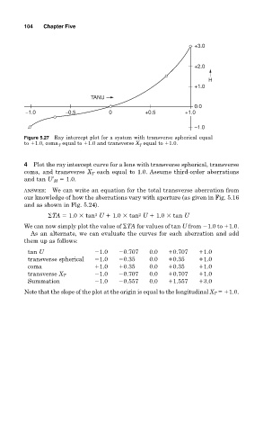
Figure 5.27 Ray intercept plot for a system with transverse spherical equal
to 1.0, coma equal to 1.0 and transverse X equal to 1.0.
T
T
4 Plot the ray intercept curve for a lens with transverse spherical, transverse
coma, and transverse X T each equal to 1.0. Assume third-order aberrations
and tan U′ M 1.0.
ANSWER: We can write an equation for the total transverse aberration from
our knowledge of how the aberrations vary with aperture (as given in Fig. 5.16
and as shown in Fig. 5.24).
2
TA 1.0 tan 3 U 1.0 tan U 1.0 tan U
We can now simply plot the value of TA for values of tan U from 1.0 to 1.0.
As an alternate, we can evaluate the curves for each aberration and add
them up as follows:
tan U 1.0 0.707 0.0 0.707 1.0
transverse spherical 1.0 0.35 0.0 0.35 1.0
coma 1.0 0.35 0.0 0.35 1.0
1.0 0.707 0.0 0.707 1.0
transverse X T
Summation 1.0 0.557 0.0 1.557 3.0
Note that the slope of the plot at the origin is equal to the longitudinal X T 1.0.