Page 213 - Numerical Analysis Using MATLAB and Excel

Chapter 5 Differential Equations, State Variables, and State Equations

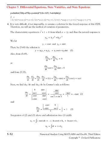
y=dsolve('D2y+2*Dy+y=cos(2*t)/2+1/2'); f=simple(y)

f =
-3/50*cos(2*t)+2/25*sin(2*t)+1/2+C1*exp(-t)+C2*exp(-t)*t
4. It is very difficult, if not impossible, to assume a solution for the forced response of this ODE.
Therefore, we will use the method of variation of parameters.

2
The characteristic equation is s + 1 = 0 from which s = j ± and thus the natural response is

jt
y N = k e + k e j – t
2
1
We let
y = cos t and y = sin t
1
2
Then, by (5.68) the solution is
y = u y + u y = u cos + u sin t (1)
t
2 2
2
1 1
1
Also, from (5.69),
du du
1
2
--------y + --------y = 0
dt 1 dt 2
or
du du
2
1
t
-------- cos + -------- sin = 0
t
dt dt
and from (5.70),
du dy du dy du du
1
2
2
1
1
(
)
⋅
⋅
)
-------- -------- + -------- -------- = ft() = -------- – sin t + -------- cos( 2 t = sec t
dt dt dt dt dt dt
Next, we find du dt⁄ and du ⁄ dt by Cramer’s rule as follows:
1
2
0 sin t sin t
du sec t cos t – ---------- t – tan t
cos
1
-------- = ----------------------------------------- = ------------------------------- = ------------- = – tan t (2)
dt cos t sin t cos 2 t + sin 2 t 1
– sin t cos t
and
cos t 0
du – sin t sec t 1
2
-------- = ----------------------------------------- = -- = 1 (3)
-
dt 1 1
Integration of (2) and (3) above and substitution into (1) yields
1 ∫
)
)
d
u = – ( tan t t = – – ( ln cos t + k = ln cos t + k 1
1
2 ∫
u = t d = t + k 2
5−52 Numerical Analysis Using MATLAB® and Excel®, Third Edition
Copyright © Orchard Publications