Page 216 - Numerical Analysis Using MATLAB and Excel

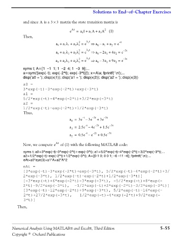
Solutions to End−of−Chapter Exercises

and since is a 3 × 3 matrix the state transition matrix is
A
At 2
e = a I + a A + a A (1)
1
2
0
Then,
2
1
a + a λ + a λ = e λ t ⇒ a – a + a = e t –
2
1
0
1
2
1
0
1
2
2
a + a λ + a λ = e λ t ⇒ a – 2a + 4a = e – 2t
1
2
2
1
0
2
0
2
2
3
a + a λ + a λ = e λ t ⇒ a – 3a + 9a = e – 3t
1
2
2 3
0
0
1 3
syms t; A=[1 −1 1; 1 −2 4; 1 −3 9];...
a=sym('[exp(−t); exp(−2*t); exp(−3*t)]'); x=A\a; fprintf(' \n');...
disp('a0 = '); disp(x(1)); disp('a1 = '); disp(x(2)); disp('a2 = '); disp(x(3))
a0 =
3*exp(-t)-3*exp(-2*t)+exp(-3*t)
a1 =
5/2*exp(-t)-4*exp(-2*t)+3/2*exp(-3*t)
a2 =
1/2*exp(-t)-exp(-2*t)+1/2*exp(-3*t)
Thus,
t –
a = 3e – 3e – 2t + 3e – 3t
0
t –
a = 2.5e – 4e – 2t + 1.5e – 3t
1
t –
a = 0.5e – e – 2t + 0.5e – 3t
2
Now, we compute e At of (1) with the following MATLAB code:
syms t; a0=3*exp(−t)−3*exp(−2*t)+exp(−3*t); a1=5/2*exp(−t)−4*exp(−2*t)+3/2*exp(−3*t);...
a2=1/2*exp(−t)−exp(−2*t)+1/2*exp(−3*t); A=[0 1 0; 0 0 1; −6 −11 −6]; fprintf(' \n');...
eAt=a0*eye(3)+a1*A+a2*A^2
eAt =
[3*exp(-t)-3*exp(-2*t)+exp(-3*t), 5/2*exp(-t)-4*exp(-2*t)+3/
2*exp(-3*t), 1/2*exp(-t)-exp(-2*t)+1/2*exp(-3*t)]
[-3*exp(-t)+6*exp(-2*t)-3*exp(-3*t), -5/2*exp(-t)+8*exp(-
2*t)-9/2*exp(-3*t), -1/2*exp(-t)+2*exp(-2*t)-3/2*exp(-3*t)]
[3*exp(-t)-12*exp(-2*t)+9*exp(-3*t), 5/2*exp(-t)-16*exp(-
2*t)+27/2*exp(-3*t), 1/2*exp(-t)-4*exp(-2*t)+9/2*exp(-
3*t)]
Then,

Numerical Analysis Using MATLAB® and Excel®, Third Edition 5−55

Copyright © Orchard Publications