Page 221 - Numerical Analysis Using MATLAB and Excel

Chapter 6 Fourier, Taylor, and Maclaurin Series

2π
)
)
Figure 6.3. Graphical proof of ∫ ( sin mt sin nt t = 0 for m = 2 and n = 3
(
d
0
Also, if and are different integers, then,
n
m
2π
∫ ( cos mt cos nt t = 0 (6.7)
)
(
)
d
0
since
)
-- cos[
( cos x cos y = 1 - ( x + y + ( cos x y ] – )
)
)
(
2
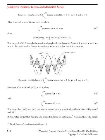
The integral of (6.7) can also be confirmed graphically as shown in Figure 6.4, where m = 2 and
n = 3 . We observe that the net shaded area above and below the time axis is zero.
⋅
cos 3x cos 2x cos 2x cos 3x

2π
(
)
)
Figure 6.4. Graphical proof of ∫ ( cos mt cos nt t = 0 for m = 2 and n = 3
d
0
However, if in (6.6) and (6.7), m = n , then,
2π
2
∫ ( sin mt d = π (6.8)
)
t
0
and
2π
∫ ( cos mt d = π (6.9)
2
)
t
0
The integrals of (6.8) and (6.9) can also be seen to be true graphically with the plots of Figures 6.5
and 6.6.
*
It was stated earlier that the sine and cosine functions are orthogonal to each other. The simpli-

* We will discuss orthogonal functions in Chapter 14

6−4 Numerical Analysis Using MATLAB® and Excel®, Third Edition
Copyright © Orchard Publications