Page 222 - Numerical Analysis Using MATLAB and Excel

Evaluation of the Coefficients

fication obtained by application of the orthogonality properties of the sine and cosine functions,
becomes apparent in the discussion that follows.

2
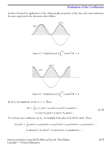
sin x
sin x

2π
2
Figure 6.5. Graphical proof of ∫ ( sin mt d = π
)
t
0

2
cos x

cos x

2π
2
)
Figure 6.6. Graphical proof of ∫ ( cos mt d = π
t
0
In (6.1), for simplicity, we let ω = 1 . Then,

1
-
ft() = --a + a cos + a cos 2t + a cos 3t + a cos 4t + …
t
2 0 1 2 3 4 (6.10)
t
+ b sin + b sin 2t + b sin 3t + b sin 4t + …
1
4
2
3
To evaluate any coefficient, say b 2 , we multiply both sides of (6.10) by sin 2t . Then,
1
ft()sin 2t = ---a sin 2t + a cos tsin 2t + a cos 2tsin 2t + a cos 3tsin 2t + a cos 4tsin 2t + …
2 0 1 2 3 4
(
b sin tsin 2t + b sin 2t ) 2 + b sin 3tsin 2t + b sin 4tsin 2t + …
2
3
4
1
Numerical Analysis Using MATLAB® and Excel®, Third Edition 6−5
Copyright © Orchard Publications