Page 220 - Numerical Analysis Using MATLAB and Excel

Evaluation of the Coefficients

1
)
sin xcos y = -- sin[ - ( x + y + ( sin x y ] – )
2
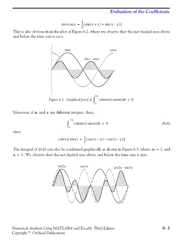
This is also obvious from the plot of Figure 6.2, where we observe that the net shaded area above
and below the time axis is zero.

sin x cos x

⋅
sin x cos x

2π
(
)
Figure 6.2. Graphical proof of ∫ ( sin mt cos nt t = 0
)
d
0
Moreover, if and are different integers, then,
n
m
2π
∫ ( sin mt sin nt t = 0 (6.6)
(
)
)
d
0
since
)
(
)
( sin x sin y = 1 - ( x – y – ( cos x y ] – )
-- cos[
)
2
The integral of (6.6) can also be confirmed graphically as shown in Figure 6.3, where m = 2 and
n = 3 . We observe that the net shaded area above and below the time axis is zero.
sin 2x sin 3x sin 2x sin 3x
⋅

Numerical Analysis Using MATLAB® and Excel®, Third Edition 6−3
Copyright © Orchard Publications