Page 273 - Numerical Analysis Using MATLAB and Excel

Chapter 6 Fourier, Taylor, and Maclaurin Series

A
⎛
--e
-
---- +
ft() = A ----- … – 1 – j3ωt – e – jωt + e jωt + 1 j3ωt + … ⎞
-
--e
2 jπ ⎝ 3 3 ⎠
The minus (−) sign of the first two terms within the parentheses results from the fact that
⁄
⁄
C – n = C ∗ . For instance, since C = 2A jπ , it follows that C – 1 = C ∗ = – 2A jπ . We
1
1
n
observe that ft() is complex, as expected, since there is no symmetry.
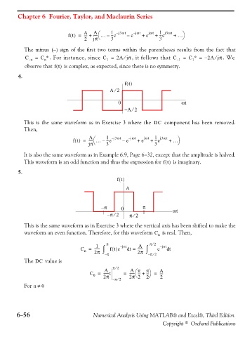
4.
ft()
⁄
A2
0 ωt
⁄
– A 2
This is the same waveform as in Exercise 3 where the DC component has been removed.
Then,
A ⎛ 1 – j3ωt – jωt jωt 1 j3ωt ⎞
-
-
ft() = ----- … – --e – e + e + --e + …
jπ ⎝ 3 3 ⎠
It is also the same waveform as in Example 6.9, Page 6−32, except that the amplitude is halved.
This waveform is an odd function and thus the expression for ft() is imaginary.

5.
ft()
A

– π 0 π ωt
⁄
– π 2 π 2
⁄
This is the same waveform as in Exercise 3 where the vertical axis has been shifted to make the
waveform an even function. Therefore, for this waveform C n is real. Then,

1 π – jnt A π 2⁄ – jnt
C = ------ ∫ π ft()e t d = ------ ∫ ⁄ e t d
n
2π
2π
The DC value is – – π 2
A π 2⁄ A π π⎞ A
⎛
C = ------t = ------ --- + --- = ----
⎠
⎝
2π
0
⁄
– π 2 2π 2 2 2
For n ≠ 0

6−56 Numerical Analysis Using MATLAB® and Excel®, Third Edition
Copyright © Orchard Publications