Page 294 - Numerical Analysis Using MATLAB and Excel

Chapter 7 Finite Differences and Interpolation

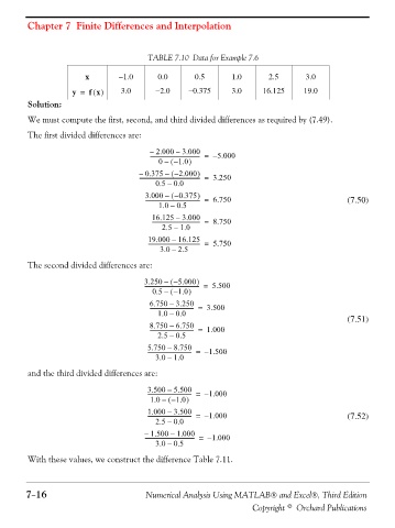
TABLE 7.10 Data for Example 7.6

x −1.0 0.0 0.5 1.0 2.5 3.0
y = f x() 3.0 −2.0 −0.375 3.0 16.125 19.0
Solution:

We must compute the first, second, and third divided differences as required by (7.49).
The first divided differences are:

– 2.000 – 3.000
------------------------------------- = – 5.000
0 ( – – 1.0 )
– 0.375 ( – – 2.000 )
--------------------------------------------- = 3.250
0.5 – 0.0
3.000 ( – – 0.375 )
----------------------------------------- = 6.750 (7.50)
1.0 – 0.5
16.125 – 3.000
------------------------------------ = 8.750
–
2.5 1.0
19.000 16.125
–
--------------------------------------- = 5.750
3.0 2.5
–
The second divided differences are:
)
3.250 ( ----------------------------------------- = 5.500
–
–
5.000
0.5 ( – – 1.0 )
–
6.750 3.250 3.500
--------------------------------- =
1.0 0.0
–
(7.51)
8.750 6.750 1.000
–
--------------------------------- =
2.5 0.5
–
–
5.750 8.750
--------------------------------- = – 1.500
–
3.0 1.0
and the third divided differences are:
3.500 – 5.500 – 1.000
--------------------------------- =
1.0 – – ( 1.0 )
1.000 – 3.500 – 1.000 (7.52)
--------------------------------- =
2.5 – 0.0
– 1.500 – 1.000 – 1.000
------------------------------------- =
3.0 – 0.5
With these values, we construct the difference Table 7.11.

7−16 Numerical Analysis Using MATLAB® and Excel®, Third Edition
Copyright © Orchard Publications