Page 299 - Numerical Analysis Using MATLAB and Excel

Gregory−Newton Backward Interpolation Method

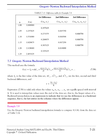
TABLE 7.13 Difference table for Example 7.8

1st Difference 2nd Difference 3rd Difference

x fx() fx x,( 0 1 ) fx x x ) ( 0 , 1 , 2 fx x x x ) ( 0 , 1 , 2 , 3
1.00 1.000000
0.257625
1.05 1.257625 0.015750
0.273375 0.000750
1.10 1.531000 0.016500
0.289875 0.000750
1.15 1.820875 0.017250
0.307125 0.000750
1.20 2.128000 0.018000
0.325125
1.25 2.453125

7.7 Gregory−Newton Backward Interpolation Method

This method uses the formula
(
(
)
(
rr + 1 ) 2 rr + 1 r + 2 ) 3
fx() = f + rΔf – 1 + ------------------Δ f – 2 + -----------------------------------Δ f – 3 + … (7.58)
0
3!
2!
2
3
where is the first value of the data set, Δf – 1 , Δ f – 2 , and Δ f – 3 are the first, second and third
f
0
backward differences, and
( x – x )
1
r = -------------------
h
Expression (7.58) is valid only when the values x x x … x, 0 1 , 2 , , n are equally spaced with interval
h . It is used to interpolate values near the end of the data set, that is, the larger values of . x
Backward interpolation is an expression to indicate that we use the differences in a backward
sequence, that is, the last entries on the columns where the differences appear.

Example 7.9
Use the Gregory−Newton backward interpolation formula to compute f1.18( ) from the data set
of Table 7.14.

Numerical Analysis Using MATLAB® and Excel®, Third Edition 7−21
Copyright © Orchard Publications