Page 297 - Numerical Analysis Using MATLAB and Excel

Gregory−Newton Forward Interpolation Method

A B C D E F G H I J K L
1 Lagrange's Interpolation Method
2 Numer. Denom. Division
3 Interpol. at x= 2 Partial Partial of Partial
4 Prods Prods Prods
5 x f(x) x-x 1 x-x 2 x-x 3 x-x 4 x-x 5 f(x 0 )
6 x 0 -1.00 3.000 2.000 1.500 1.000 -0.500 -1.000 3.000 4.500
7 x 1 0.00 -2.000 x 0 -x 1 x 0 -x 2 x 0 -x 3 x 0 -x 4 x 0 -x 5 -0.107
8 x 2 0.50 -0.375 -1.000 -1.500 -2.000 -3.500 -4.000 -42.000
9 x 3 1.00 3.000 x-x 0 x-x 2 x-x 3 x-x 4 x-x 5 f(x 1 )
10 x 4 2.50 16.125 3.000 1.500 1.000 -0.500 -1.000 -2.000 -4.500
11 x 5 3.00 19.000 x 1 -x 0 x 1 -x 2 x 1 -x 3 x 1 -x 4 x 1 -x 5 -1.200
12 1.000 -0.500 -1.000 -2.500 -3.000 3.750
13 x-x 0 x-x 1 x-x 3 x-x 4 x-x 5 f(x 2 )
14 3.000 2.000 1.000 -0.500 -1.000 -0.375 -1.125
15 x 2 -x 0 x 2 -x 1 x 2 -x 3 x 2 -x 4 x 2 -x 5 0.600
16 1.500 0.500 -0.500 -2.000 -2.500 -1.875
17 x-x 0 x-x 1 x-x 2 x-x 4 x-x 5 f(x 3 )
18 3.000 2.000 1.500 -0.500 -1.000 3.000 13.500
19 x 3 -x 0 x 3 -x 1 x 3 -x 2 x 3 -x 4 x 3 -x 5 4.500
20 2.000 1.000 0.500 -1.500 -2.000 3.000
21 x-x 0 x-x 1 x-x 2 x-x 3 x-x 5 f(x 4 )
22 3.000 2.000 1.500 1.000 -1.000 16.125 -145.125
23 x 4 -x 0 x 4 -x 1 x 4 -x 2 x 4 -x 3 x 4 -x 5 11.057
24 3.500 2.500 2.000 1.500 -0.500 -13.125
25 x-x 0 x-x 1 x-x 2 x-x 3 x-x 4 f(x 5 )
26 3.000 2.000 1.500 1.000 -0.500 19.000 -85.500
27 x 5 -x 0 x 5 -x 1 x 5 -x 2 x 5 -x 3 x 5 -x 4 -2.850
28 4.000 3.000 2.500 2.000 0.500 30.000
29
30 f(2)= Sum= 12
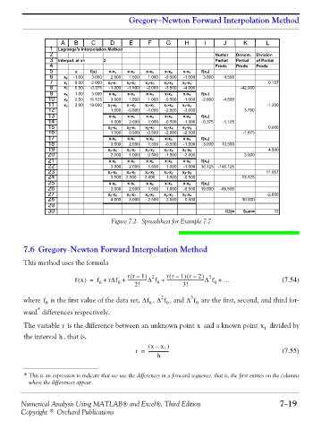
Figure 7.2. Spreadsheet for Example 7.7

7.6 Gregory−Newton Forward Interpolation Method
This method uses the formula

(
)
(
(
rr – 1 ) 2 rr – 1 r – 2 ) 3
fx() = f + rΔf + ------------------Δ f + ----------------------------------Δ f + … (7.54)
0
0
0
0
3!
2!
2 3
f
where is the first value of the data set, Δf 0 , Δ f 0 , and Δ f 0 are the first, second, and third for-
0
*
ward differences respectively.
The variable is the difference between an unknown point and a known point x 1 divided by
r
x
the interval , that is,
h
( x – x )
1
r = ------------------- (7.55)
h
* This is an expression to indicate that we use the differences in a forward sequence, that is, the first entries on the columns
where the differences appear.
Numerical Analysis Using MATLAB® and Excel®, Third Edition 7−19
Copyright © Orchard Publications