Page 302 - Numerical Analysis Using MATLAB and Excel

Chapter 7 Finite Differences and Interpolation

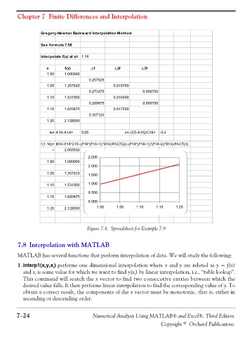
Gregory-Newton Backward Interpolation Method

See formula 7.58

Interpolate f(x) at x= 1.18

x f(x) Δf Δ2f Δ3f
1.00 1.000000
0.257625
1.05 1.257625 0.015750
0.273375 0.000750
1.10 1.531000 0.016500
0.289875 0.000750
1.15 1.820875 0.017250
0.307125
1.20 2.128000

h= A16-A14= 0.05 r= (C5-A16)/C18= -0.4

f(1.18)= B16+F18*C15+(F18*(F18+1)*D14)/FACT(2)+(F18*(F18+1)*(F18+2)*E13)/FACT(3)
= 2.003032
2.500
1.00 1.000000
2.000
1.05 1.257625 1.500

1.10 1.531000 1.000
0.500
1.15 1.820875
0.000
1.20 2.128000 1.00 1.05 1.10 1.15 1.20

Figure 7.4. Spreadsheet for Example 7.9

7.8 Interpolation with MATLAB

MATLAB has several functions that perform interpolation of data. We will study the following:
1. interp1(x,y,x ) performs one dimensional interpolation where x and y are related as y = f(x)
i
and x is some value for which we want to find y(x ) by linear interpolation, i.e., “table lookup”.
i
i
This command will search the x vector to find two consecutive entries between which the
desired value falls. It then performs linear interpolation to find the corresponding value of y. To
obtain a correct result, the components of the x vector must be monotonic, that is, either in
ascending or descending order.

7−24 Numerical Analysis Using MATLAB® and Excel®, Third Edition
Copyright © Orchard Publications