Page 307 - Numerical Analysis Using MATLAB and Excel

Interpolation with MATLAB

%
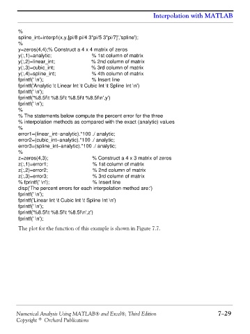
spline_int=interp1(x,y,[pi/8 pi/4 3*pi/5 3*pi/7]','spline');
%
y=zeros(4,4);% Construct a 4 x 4 matrix of zeros
y(:,1)=analytic; % 1st column of matrix
y(:,2)=linear_int; % 2nd column of matrix
y(:,3)=cubic_int; % 3rd column of matrix
y(:,4)=spline_int; % 4th column of matrix
fprintf(' \n'); % Insert line
fprintf('Analytic \t Linear Int \t Cubic Int \t Spline Int \n')
fprintf(' \n');
fprintf('%8.5f\t %8.5f\t %8.5f\t %8.5f\n',y')
fprintf(' \n');
%
% The statements below compute the percent error for the three
% interpolation methods as compared with the exact (analytic) values
%
error1=(linear_int−analytic).*100 ./ analytic;
error2=(cubic_int−analytic).*100 ./ analytic;
error3=(spline_int−analytic).*100 ./ analytic;
%
z=zeros(4,3); % Construct a 4 x 3 matrix of zeros
z(:,1)=error1; % 1st column of matrix
z(:,2)=error2; % 2nd column of matrix
z(:,3)=error3; % 3rd column of matrix
% fprintf(' \n'); % Insert line
disp('The percent errors for each interpolation method are:')
fprintf(' \n');
fprintf('Linear Int \t Cubic Int \t Spline Int \n')
fprintf(' \n');
fprintf('%8.5f\t %8.5f\t %8.5f\n',z')
fprintf(' \n');
The plot for the function of this example is shown in Figure 7.7.

Numerical Analysis Using MATLAB® and Excel®, Third Edition 7−29
Copyright © Orchard Publications