Page 308 - Numerical Analysis Using MATLAB and Excel

Chapter 7 Finite Differences and Interpolation

5
y=cos (x)
1
0.8
0.6
0.4
0.2
y 0
-0.2
-0.4
-0.6
-0.8
-1
0 1 2 3 4 5 6
x
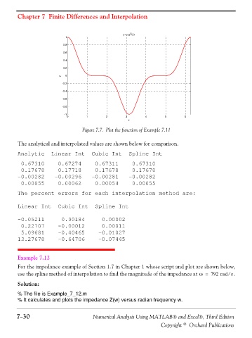
Figure 7.7. Plot the function of Example 7.11

The analytical and interpolated values are shown below for comparison.

Analytic Linear Int Cubic Int Spline Int
0.67310 0.67274 0.67311 0.67310
0.17678 0.17718 0.17678 0.17678
-0.00282 -0.00296 -0.00281 -0.00282
0.00055 0.00062 0.00054 0.00055
The percent errors for each interpolation method are:

Linear Int Cubic Int Spline Int

-0.05211 0.00184 0.00002
0.22707 -0.00012 0.00011
5.09681 -0.40465 -0.01027
13.27678 -0.64706 -0.07445

Example 7.12
For the impedance example of Section 1.7 in Chapter 1 whose script and plot are shown below,

use the spline method of interpolation to find the magnitude of the impedance at ω = 792 rad . s ⁄
Solution:

% The file is Example_7_12.m
% It calculates and plots the impedance Z(w) versus radian frequency w.

7−30 Numerical Analysis Using MATLAB® and Excel®, Third Edition
Copyright © Orchard Publications