Page 306 - Numerical Analysis Using MATLAB and Excel

Chapter 7 Finite Differences and Interpolation

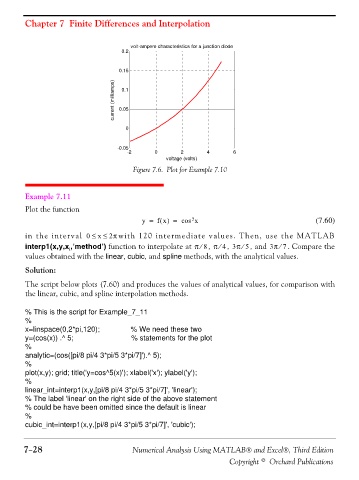
volt-ampere characteristics for a junction diode
0.2

0.15
current (milliamps) 0.05
0.1

0

-0.05
-2 0 2 4 6
voltage (volts)
Figure 7.6. Plot for Example 7.10

Example 7.11

Plot the function
y = f x() = cos 5 x (7.60)

in the interval 0 ≤≤ 2π with 120 intermediate values. Then, use the MATLAB
x
interp1(x,y,x ,’method’) function to interpolate at π 8⁄ , π , 4 ⁄ 3π 5 , and 3π 7⁄ . Compare the
⁄
i
values obtained with the linear, cubic, and spline methods, with the analytical values.
Solution:

The script below plots (7.60) and produces the values of analytical values, for comparison with
the linear, cubic, and spline interpolation methods.

% This is the script for Example_7_11
%
x=linspace(0,2*pi,120); % We need these two
y=(cos(x)) .^ 5; % statements for the plot
%
analytic=(cos([pi/8 pi/4 3*pi/5 3*pi/7]').^ 5);
%
plot(x,y); grid; title('y=cos^5(x)'); xlabel('x'); ylabel('y');
%
linear_int=interp1(x,y,[pi/8 pi/4 3*pi/5 3*pi/7]', 'linear');
% The label 'linear' on the right side of the above statement
% could be have been omitted since the default is linear
%
cubic_int=interp1(x,y,[pi/8 pi/4 3*pi/5 3*pi/7]', 'cubic');

7−28 Numerical Analysis Using MATLAB® and Excel®, Third Edition
Copyright © Orchard Publications